
2 Data Dalliances (WIP)
The first step to data analysis is, in fact, data. While this may seem obvious, statistics textbooks often dodge this detail. Discussions of regression analysis often begin with a statement like:
“Let \(X\) be the \(n x p\) design matrix of independent variables…”
but in practice this statement is as absurd as writing a book about how to win a basketball game, assuming your team already has a 20 point lead with 1 minute left to play.
It’s very convenient but typically incorrect to assume that the data we happen to have is the ideal (or, more humbly, sufficient) data for the questions we wish to analyze. The specific vagaries of data vary greatly by domain, but a commonality across many fields (such as political science, economics, epidemiology, and market research) is that we are often called to work with found data (or, more formally, “observational data”) from administrative sources or production systems. In contrast to artisanally crafted data experimental data (like the carefully controlled agricultural experiments which motivated many early methods developments in statistics), this data was generated neither by us nor for us. To quote Angela Bassa, the head of data science at an e-commerce company: “Data isn’t ground truth. Data are artifacts of systems” (Bassa 2017).
The analytical implications of observational versus experimental data are well explored in the field of causal inference (which we will discuss some in Chapter 6 and Chapter 7). However, this distinction has implications far earlier in the data analysis process, as well. To name a few:
- Records and fields many not represent the entities or measures most conducive to analysis
- Data collection methods may capture a different subset of events or do so at a different frequency than we expected, leading to systemic biases
- Data movement between systems can insert errors (or, at minimum, challenges to our intuition)
- Data transformations may be fragile or transient, reflecting the primary purpose of the system not our unrelated analytical use
In this chapter, we will explore data structures and the full data generating process to better understand how different types of data challenges emerge. In doing so, we will hone sharper intuition for how our data can deceive us and what to watch out for when beginning an analysis.
2.1 Preliminaries
Before we begin our exploration of data dalliances, we must first establish a baseline understanding of data structure, data production, and data quality.
2.1.1 Data Structure Basics
2.1.1.1 Relational Data Structure
Understanding the content and structure of the data you are using is a critical prerequisite to analysis. In this book, we focus on tabular, structured data like one might find in an Excel spreadsheet or relational database.1
In particular, many tools work best with what R developer Hadley Wickham describes as “tidy data” (Wickham 2014). Namely:
- Each variable forms a column
- Each observation forms a row
- Each type of observational unit forms a table
This is analogous to how one generally finds data arranged in a database and how statisticians are used to conceptualizing it. For example, the design matrix of a linear model consists of one column of data for each independent variable to be included in the model and one row for each observation.2 As Wickham points out, this is also similar to what is called “3rd normal form” in the world of relational database management systems.
Using this data structure is valuable not only because it is similar to what many modern data tools expect, but also because it provides us a framework to think critically about what defined each observation and each variable in our dataset.
2.1.1.2 Schemas
The first part of the definition of tidy data references variables in columns. These variables in turn consist of three main parts:
- A column name used to access and manipulate that data
- A data type used to store that data (e.g. and integer format or data format)
- A definition used to denote what that field represents in the real-world
Column names are always explicit. In a database or a language like R and python, the data type is also explicit.3 Ideally, the definition is explicitly defined in metadata or a data dictionary, but sometimes this may be implicit.
2.1.2 Data Production Processes
In statistical modeling we discuss the data generating process: we can build models that describe the mechanisms that create our observations. We can broaden this notion to think about the generating process of each of these steps of data production.
Regardless of the type of data (experimental, observational, survey, etc.), there are generally four main steps to production: collection, extraction, loading, and transformation.4
- Collect: The way in which signals from the real world are captured as data. This could include logging (e.g. for web traffic or system monitoring), sensors (e.g. temperature collection), surveys, and more
- Extract: The process of removing data from the place in which it was originally captured in preparation of moving it somewhere in which analysis can be done
- Load: The process of loading the extracted data to its final destination
- Transform: The process of modeling and transforming data so that its structure is useful for analysis and its variables are interpretable
To better theorize about data quality issues, it’s useful to think of four DGPs (as shown in Figure 2.1): the real-world DGP, the data collection/extraction DGP5, the data loading DGP, and the data transformation DGP.
2.1.2.1 E-Commerce Data Example
For example, consider the role of each of these four DGPs for e-commerce data:
- Real-world DGP: Supply, demand, marketing, and a range of factors motivate a consumer to visit a website and make a purchase
- Data collection DGP: Parts of the website are instrumented to log certain customer actions. This log is then extracted from the different operational system (login platforms, payment platforms, account records) to be used for analysis
- Data loading DGP: Data recorded by different systems is moved to a data warehouse for further processing through some sort of manual, scheduled, or orchestrated job. These different systems may make data available at different frequencies.
- Data transformation DGP: To arrive at that final data presentation requires creating a data model to describe domain-specific attributes with key variables crafted with data transformations
2.1.2.2 Subway Data Example
Or, consider the role of each of these four DGPs for subway ridership data6:
- Real-world DGP: Riders are motivated to use public transportation to commute, run errands, or visit friends. Different motivating factors may cause different weekly and annual seasonality
- Data collection DGP: To ride the subway, riders go to a station and enter and exit through turnstiles. The mechanical rotation of the turnstile caused by a rider passing through is recorded
- Data loading DGP: Data recorded at each turnstile is collected through a centralized computer system at the station. Once a week, each station uploads a flat file of this data to a data lake owned by the city’s Department of Transportation
- Data transformation DGP: Turnstiles from different companies may have different data formats. Transformation may include harmonizing disparate sources, coding system-generated codes (e.g. Station XYZ) to semantically meaningful names (e.g. Main Street Station), and publishing a final unified representation across stations and across time
Throughout this chapter, we’ll explore how understanding key concepts about each of these DGPs can help guide our intuition on where to look for problems.
2.1.3 Data Quality Dimension
To guide our discussion of how data production can affect aspects of data quality, we need a guiding definition of data quality. This is challenging because data quality is subjective and task-specific. It matters much more if data is “fit for purpose” and operates in a way that is transparent to its users moreso than meeting some preordained quality standard.
Regardless, it’s useful for our discussion to think about general dimensions of data quality. Here, we will rely on six dimensions of data quality outlined by Data Management Association (“Six Dimensions of Data Quality Assessment” 2020). Their official definitions are:
- Completeness: The proportion of stored data against the potential of “100% completeâ€
- Uniqueness: Nothing will be recorded more than once based upon how that thing is identified. It is the inverse of an assessment of the level of duplication
- Timeliness: The degree to which data represent reality from the required point in time
- Validity: Data are valid if it conforms to the syntax (format, type, range) of its definition
- Accuracy: The degree to which data correctly describes the “real world” object or event being described.
- Consistency: The absence of difference, when comparing two or more representations of a thing against a definition
2.1.4 Questions to Ask (TODO)
Our goal of understanding data is to ensure can assess its data quality and fit for our purpose. Understanding both its structure and its production process helps to accomplish this.
2.2 Data Collection
Data collection is the process of capturing and digitizing something in the real-world.
One of the tricky nuances of data collection is understanding what precisely is getting captured and logged in the first place. No matter how robust the sensors, loggers, or other mechanisms are that record our dataset, that data is still unfit for its purpose so long as the analyst does not fully understand what it represents. In the next section, we will see how what data gets collected (and our understanding of it) can alter our notions of data completion and how we must handle it in our computations.
Data can be collected in many different ways such as:
- Direct measurement: A researcher directly engages with each observation to measure certain characteristics
- Self-report: Information is requested from individual (human) observations who provide information
- Logging: Information is captured with proactively-configured sensors or logs which record certain behaviors
- Residue: Data is produced as an artifact of an operational system but is then re-purposed for analysis
Each approach is best suited for different circumstances and has unique benefits and challenges. For example:
- Direct measurement: Can lead to measurement error. If multiple people are collecting this data, these errors could be correlated within each researcher and break the independence of observations.
- Self-report: Can easily become biased by factors such as what type of people are inclined to respond to the request for information and if they feel obligated to provide socially desirable answers
- Logging: Can suffer from overly specific or outdated definitions of events
- Residue: Can behave in unexpected ways since the data was collected for purposes different from analysis
Regardless of the specifics, an important part of data collection is understanding precisely whose data (that is, what population) is getting collected. No matter how robust the sensors, loggers, or other mechanisms are, that data is still unfit for its purpose so long as the analyst does not fully understand what it represents. In the next section, we will see how what data gets collected (and our understanding of it) can alter our notions of data completeness and how we must handle it in our computations.
2.2.1 What Makes a Record (Row)
The first priority when starting to work with a dataset is understanding what a single record (row) represents and what causes it to be generated.
Consider something as simple as a login system where users must enter their credentials, endure a Captcha-like verification process to prove that they are not a robot, and enter a multi-factor authentication code. Figure 2.2 depicts such a process.
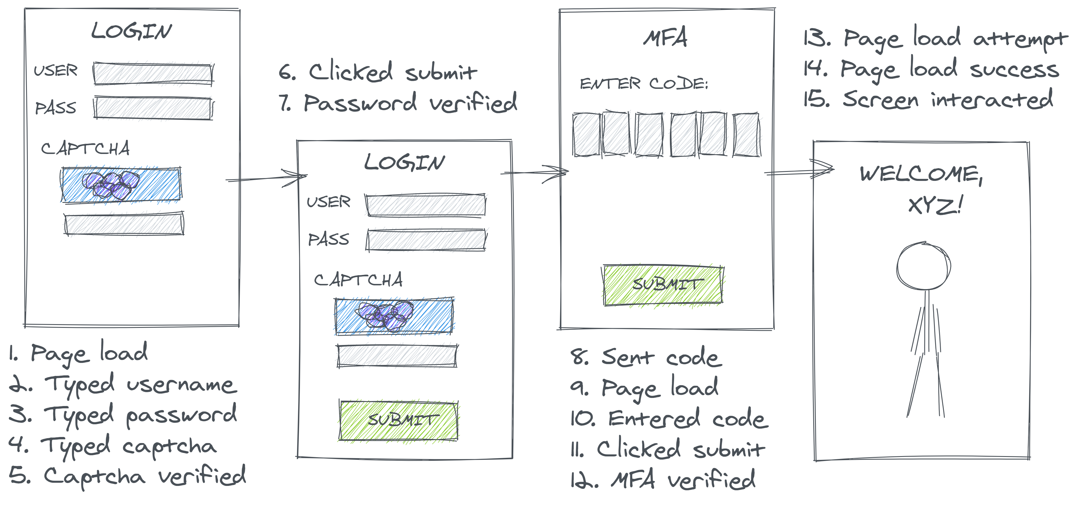
Which of these events gets collected and recorded has a significant impact on subsequent data processing. In a technical sense, no inclusion/exclusion decision here is incorrect, per se, but if the producers’ choices don’t match the consumers’ understandings, it can lead to misleading results.
For example, an analyst might seek out a logins table in order to calculate the rate of successful website logins. Reasonably enough, they might compute this rate as the sum of successful events over the total. Now, suppose two users attempt to login to their account, and ultimately, one succeeds in accessing their private information and the other doesn’t. The analyst would probably hope to compute and report a 50% login success rate. However, depending on how the data is represented, they could quite easily compute nearly any value from 0% to 100%.
As a thought experiment, we can consider what types of events might be logged:
- Per Attempt: If data is logged once per overall login attempt, successful attempts only trigger one event, but a user who forgot their password may try (and fail) to login multiple times. In the case illustrated above, that deflates the successful login rate to 25%.
- Per Event: If the logins table contains a row for every login-related event, each ‘success’ will trigger a large number of positive events and each ‘failure’ will trigger a negative event preceded by zero or more positive events. In the case illustrated below, this inflates our successful login rate to 86%.
- Per Conditional: If the collector decided to only look at downstream events, perhaps to circumvent record duplication, they might decide to create a record only to denote the success or failure of the final step in the login process (MFA). However, login attempts that failed an upstream step would not generate any record for this stage because they’ve already fallen out of the funnel. In this case, the computed rate could reach 100%
- Per Intermediate: Similarly, if the login was defined specifically as successful password verification, the computed rate could his 100% even if some users subsequently fail MFA
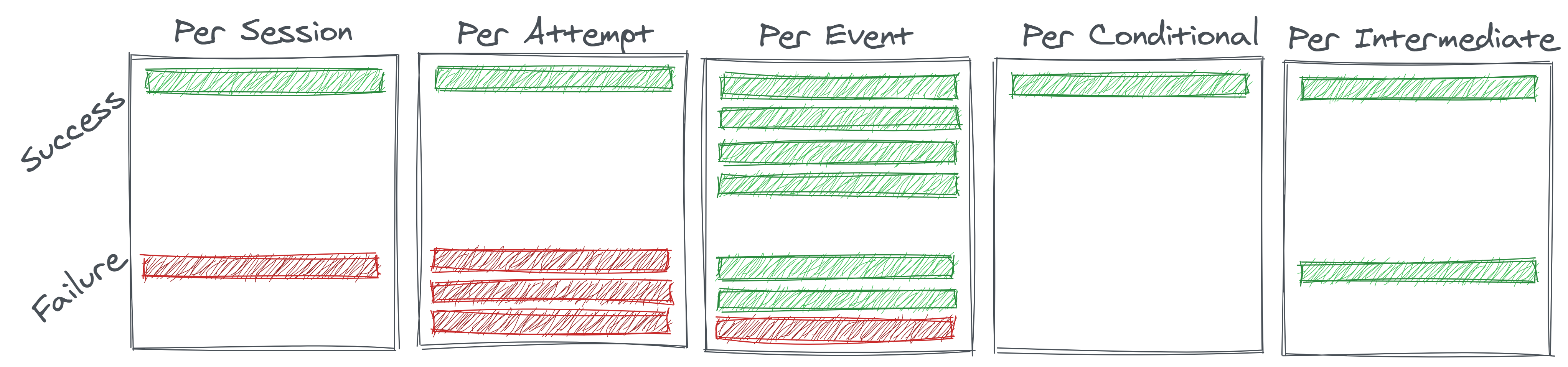
These different situations are further illustrated in Figure 2.3, and their calculations are shown in Table 2.1.
| Session | Attempt | Event | Outcome | Intermediate | |
|---|---|---|---|---|---|
| Success | 1 | 1 | 6 | 1 | 2 |
| Total | 2 | 4 | 7 | 1 | 2 |
| Rate (%) | 50 | 25 | 86 | 100 | 100 |
(Note that we did not explicitly “simulate” data here, but the workflow is largely the same. We imagine a real-world process, how that might translate into a digital representation, and created a numerical example to understand the implications. Not all simulations require fancy code; sometimes paper and a pencil or a thought experiment works just fine.)
While humans have a shared intuition of what concepts like a user, session, or login are, the act of collecting data forces us to map that intuition onto an atomic event. Any misunderstanding in precisely what that definition is can have massive impact on the perceived data quality; “per event” data will appear heavily duplicated if it is assumed to be “per session” data.
In some cases, this could be obvious to detect. If the system outputs fields that are incredibly specific (e.g. with some hyperbole, imagine a step_in_the_login_process field with values taking any of the human-readable descriptions of the fifteen processes listed in the image above), but depending how this source is organized (e.g. in contrast to above, if we only have fields like sourceid and processid with unintuitive alphanumeric encoded values) and defined, it could be nearly impossible to understand the nuances without uncovering quality metadata or talking to a data producer.
2.2.2 What Doesn’t Make a Record (Row)
Along with thinking about what does count (or gets logged), it’s equally important to understand what systemically does not generate a record. Consider users who have the intent or desire to login (motivated by a real-world DGP) but cannot find the login page, or users who load the login page but never click a button because they know that they’ve forgotten their password and see no way to request it. Often, some of these corner cases may be some of the most critical and informative (e.g. here, demonstrating some major flaws in our UI). It’s hard to computationally validate what data doesn’t exist, so conceptual data validation is critical.
2.2.3 Records versus Keys
The preceding discussion on what types of real-world observations will or will not generate records in our resulting dataset is related to but distinct from another important concept from the world of relational databases: primary keys.
Primary keys are a minimal subset of variables in a dataset than define a unique record. For example, in the previous discussion of customer logins this might consist of natural keys7 such as the combination of a session_id and a timestamp or surrogate keys8 such as a global event_id that is generated every time the system logs any event.
Understanding a table’s primary keys can be useful for many reasons. To name a few reasons, these fields are often useful for linking data from one table to another and for identifying data errors (if the uniqueness of these fields are not upheld). They also can be suggestive of the true granularity of the table.
However, simply knowing a table’s primary keys does not resolve the issues we discussed in the prior two sections. Any of the many different data collection strategies we considered are unique by session and timestamp; however, as we’ve seen, that is no guarantee that they must contain every session and timestamp in the universe of events.
2.2.4 What Defines a Variable (Column)
Just as critical as understanding what constitutes a record (row) in a dataset is understanding the precise definition of each variable (column). Superficially, this task seems easier: after all, each variable has a name which hopefully includes some semantic information. However, quite often this information can provide a false sense of security. Just because you identify a variable with a promising sounding name, that does not mean that it is the most relevant data for your analysis.
For example, consider wanting to analyze patterns in customer spend amounts across orders on an e-commerce website. You might find a table of orders with a field called amt_spend. But what might this mean?
- If the dataset is sourced from a payment processor, it likely includes the total amount billed to a customers’ credit card: including item prices less any discounts, shipping costs, taxes, etc. Alternatively, if this order was split across a gift card and a credit card, this field might only reflect the amount charged to the credit card
- If the dataset is created for Finance, it might perhaps include only the total of item prices less discounts if this best corresponded to the data the Finance team needs for revenue reporting
- Someone, somewhere, at some point might have assigned
amt_spendto the name of the variable containing gross spend (before accounting for any discounts) and there might be a different variableamt_spend_netwhich accounts for discounts applied
It’s critical to understand what each variable actually means. The upside of this is that it forces analysts to think more crisply about their research questions and what the ideal variables for their analysis would be. As we’ve seen, concepts like “spend” may seem deceptively simple, but are not unambiguous.
2.3 Data Extraction & Loading
Checking that data contains expected and only expected records (that is, completeness, uniqueness, and timeliness) is one of the most common first steps in data validation. However, the superficially simple act of loading data into a data warehouse or updating data between tables can introduce a variety of risks to data completeness which require different strategies to detect. Data loading errors can result in data that is stale, missing, duplicate, inconsistently up-to-date across sources, or complete but for only a subset of the range you think.
While the data quality principles of completeness, uniqueness, and timeliness would suggest that records should exist once and only once, the reality of many haphazard data loading process means data may appear sometime between zero and a handful of times. Data loads can occur in many different ways. For example, they might be:
No approach is free from challenges. For example, scheduled jobs risk executing before an upstream process has completed (resulting in stale or missing data); poorly orchestrated jobs may be prevented from working due to one missing dependency or might allow multiple stream to get out of sync (resulting in multisource missing data). Regardless of the method, all approaches must be carefully configured to handle failures gracefully to avoid creating duplicates, and the frequency at which they are executed may cause partial loading issues if it is incompatible with the granularity of the source data.
2.3.0.1 Data Load Failure Modes
To develop our understanding of the true data generating process and to formulate theories on how our data could be broken (and what we should validate), it is useful to understand the different ways data extraction and loading can fail.
Figure 2.4 illustrates a number of examples. Suppose that each row of boxes in the diagram represents one day of records in a table.
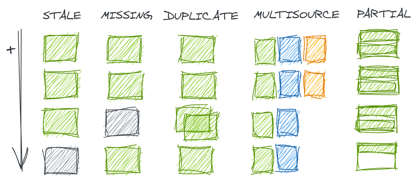
Our dataset might be susceptible to:
- Stale data occurs when the data is not as up-to-date as would be expected from is regular refresh cadence. This could happen if a manual step was skipped, a scheduled job was executed before the upstream source was available, or orchestrated data checks found errors and quarantined new records
- Missing data occurs when one data load fails but subsequent loads have succeeded
- Duplicate data occurs when one data load is executed multiple times
- Multisource missing data occurs when a table is loaded from multiple sources, and some have continued to update as expected while others have not
- Partial data occurs when a table is loaded correctly as intended by the producer but contains less data than expected by the consumer (e.g. a table loads ever 12 hours but because there is some data for a given date, the user assumes that all relevant records for that date have been loaded)
The differences in these failure modes become important when an analyst attempts to assess data completeness. One of the first approaches an analyst might consider is simply to check the min() and max() event dates in their table. However, this can only help detect stale data. To catch missing data, an analyst might instead attempt to count the number of distinct days represented in the data; to detect duplicate data, that analyst might need to count records by day and examine the pattern.
| Metric | Stale | Missing | Duplicate | Multi | Partial |
|---|---|---|---|---|---|
min(date)max(date)
|
1 3 |
1 4 |
1 4 |
1 4 |
1 4 |
count(distinct date) |
3 | 3 | 4 | 4 | 4 |
count(1) by date |
100 100 100 0 |
100 100 0 100 |
100 100 200 100 |
100 100 66 66 |
100 100 100 50 |
count(1)count(distinct PKs)
|
300 300 |
300 300 |
400 300 |
332 332 |
350 350 |
In a case like the toy example above where the correct number of rows per date is highly predictable and the number of dates is small, such eyeballing is feasible; however when the expected number of records varies day-to-day or time series are long, this approach becomes subjective, error-prone, and intractable. Additionally, it still might be hard to catch errors in multi-source data or partial loads if the lower number of records was still within the bounds of reasonable deviation for a series. These last two types deserve further exploration.
2.3.0.2 Multi-Source
A more effective strategy for assessing data completeness requires a better understanding of how data is being collected and loaded. In the case of multi-source data, one single source stopping loading may not be a big enough change to disrupt aggregate counts but could still jeopardize meaningful analysis. It would be more useful to conduct completeness checks by subgroup to identify these discrepancies.
But not any subgroup will do; the subgroup must correspond to the various data sources. For example, suppose we run an e-commerce store and wish to look at sales from the past month by category. Naturally, we might think to check the completeness of the data by category. But what if sales data is sourced from three separate locations: our Shopify site (80%), our Amazon Storefront (15%), and phone sales (5%). Unless we explicitly check completeness by channel (a dimension we don’t particularly care about for our analysis), it would be easy to miss if our data source for phone sales has stopped working or loads at a different frequency.
Another interesting aspect of multi-source data, is multiple sources can contribute either to different rows/records or different columns/variables. Table-level frequency counts won’t help us in the latter case since other sources might create the right total number of records but result in some specific fields in those records being missing or inaccurate.
2.3.0.3 Partial Loads
Partial loads really are not data errors at all, but are still important to detect since they can jeopardize an analysis. A common scenario might occur if a job loads new data every 12 hours (say, data from the morning and afternoon of day n-1 loads on day n at 12AM and 12PM, respectively). An analyst retrieving data at 11AM may be concerned to see an approximate ~50% drop in sales in the past day, despite confirming that their data looks to be “complete” since the maximum record date is, in fact, day n-1. Of course, this concern could be somewhat easily allayed if they then checked a timestamp field, but such a field might not exists or might not have been used for validation since its harder to anticipate the appropriate maximum timestamp than it is the maximum date.
2.3.0.4 Delayed or Transient Records
The interaction between choices made in the data collection and data loading phases can introduce their own sets of problems.
Consider an orders table for an e-commerce company that analysts may use to track customer orders. It might contain one record per order_id x event (placement, processing, shipment), one record per order placed, one record per order shipping, or one record per order with a status field that changes over time to denote the order’s current stage of life. Some of these options are illustrated in Figure 2.5.
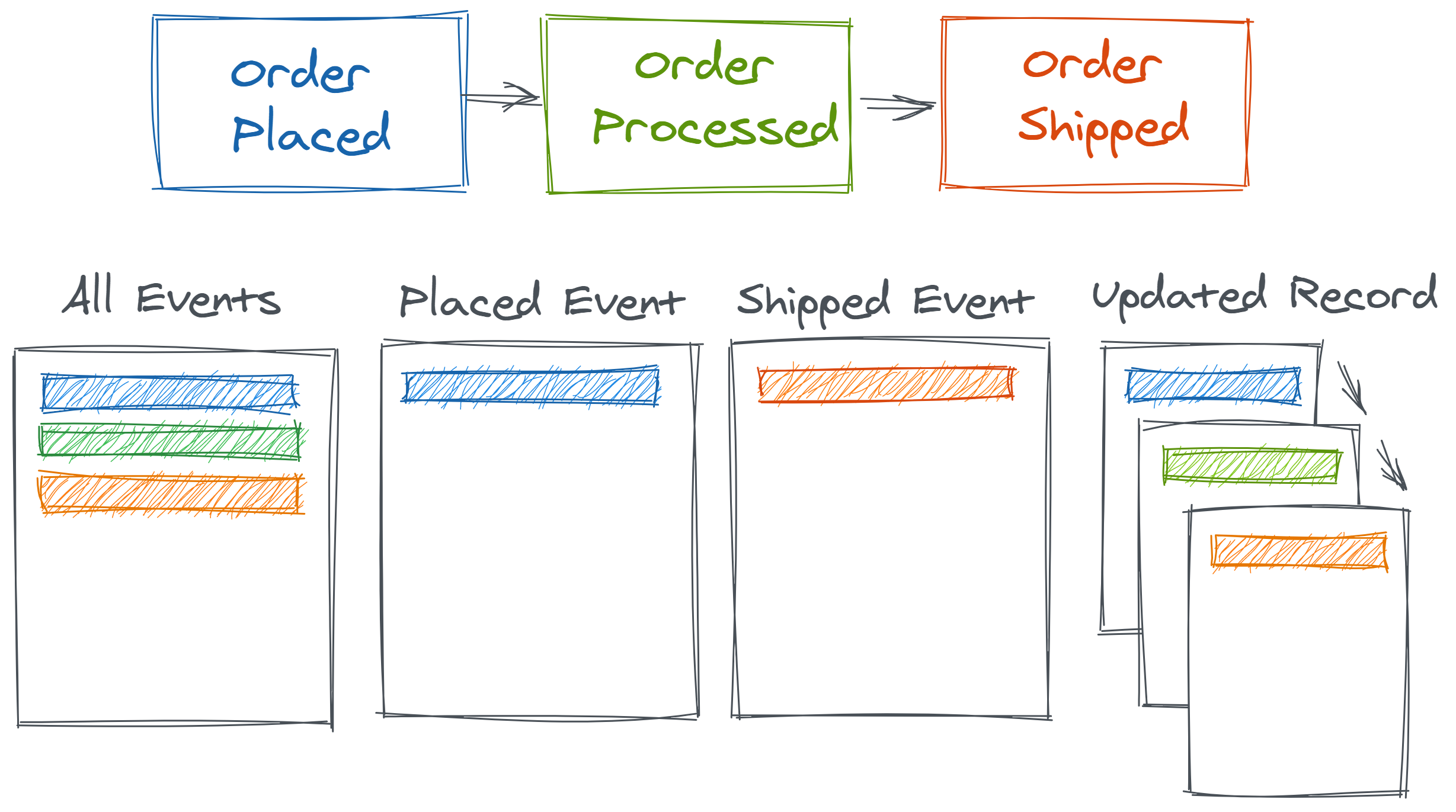
Any of these modeling choices seem reasonable and the difference between them might appear immaterial. But consider the collection choice to record and report shipped events. Perhaps this might be operationally easier if shipment come from one source system whereas orders could come from many. However, an interesting thing about shipments is that they are often lagged in a variable way from the order date.
Suppose the e-commerce company in question offers three shipping speeds at checkout. Figure 2.6 shows the range of possible shipment dates based on the order dates for the three different speeds (shown in different bars/colors).
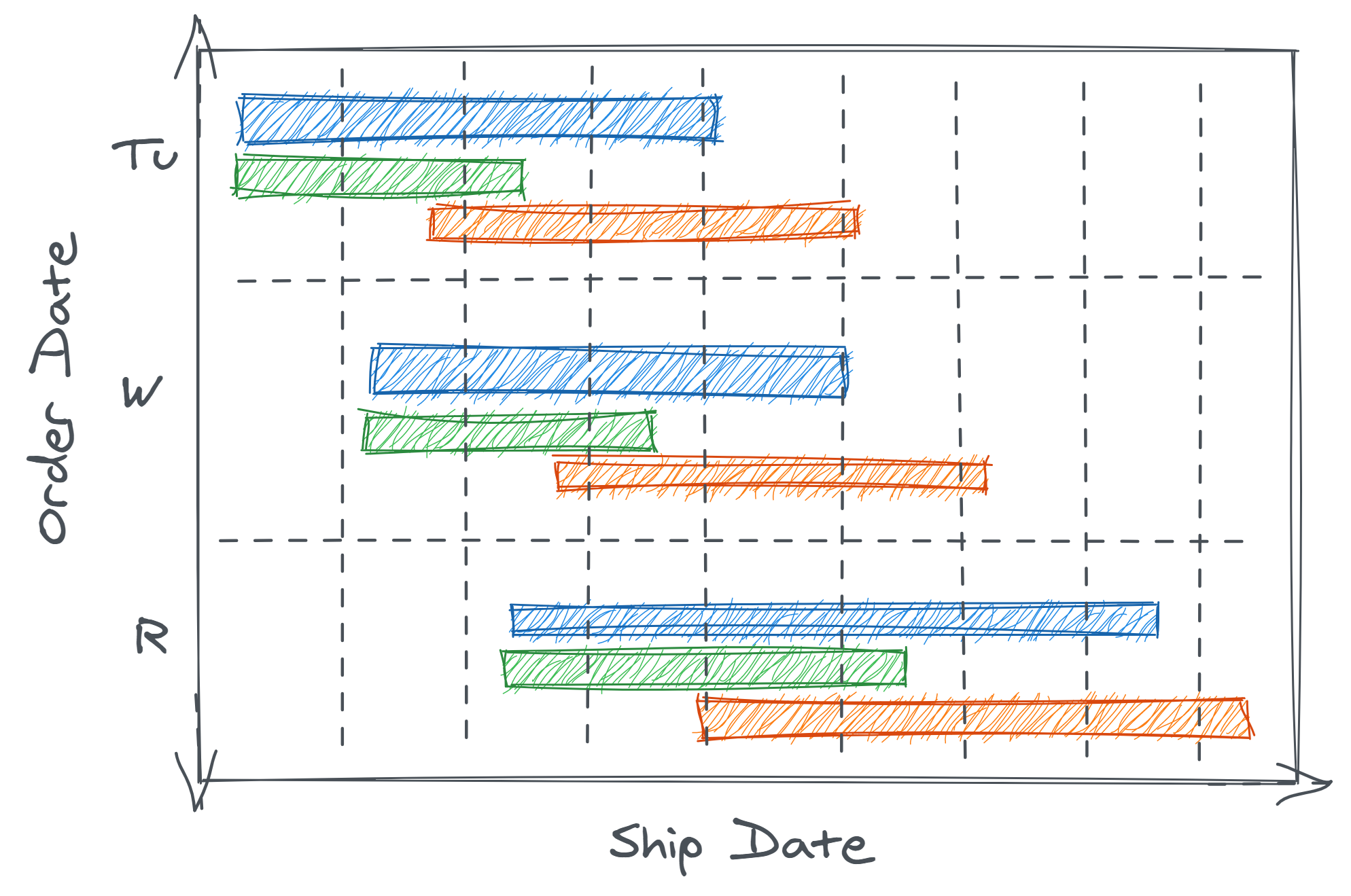
How might this effect our perceived data quality?
- Order data could appear stale or not timely since orders with a given
order_datewould only load days later once shipped - Similar to missing or multisource data, the data range in the table could lead to deceptive and incomplete data validation because some orders from a later order date might ship (and thus be logged) before all orders from a previous order date
- Put another way, we could have multiple order dates demonstrating partial data loads
- These features of the data might behave inconsistently across time due to seasonality (e.g. no shipping on weekends or federal holidays), so heuristics developed to clean the data based on a small number of observations could fail
- From an analytical perspective, orders with faster shipping would be disproportionately overrepresented in the “tail” (most recent) data. If shipping category correlated with other characteristics like total order spend, this could create an artificial trend in the data
Once again, understanding that data is collected at point of shipment and reasoning how shipment timing varies and impacts loading is necessary for successful validation.
If this thought experiment seems to vague, we can make it more concrete by mocking up a dataset with which to experiment.
In the simplest version, we will simply suppose one order is submited on each of 10 days with dates (represented for convenience as integers and not calendar dates) given by the dt_subm vector. Suppose shipping always takes three days, so we can easily calculate the shipment date (dt_ship) based on the submission date. The shipment date is the same as the date the data will be logged and loaded (dt_load).
# data simulation: single orders + deterministic ship dates ----
dt_subm <- 1:10
days_to_ship <- 3
dt_ship <- dt_subm + days_to_ship
dt_load <- dt_ship
df <- data.frame(dt_subm, dt_ship, dt_load)
head(df)
dt_subm dt_ship dt_load
1 1 4 4
2 2 5 5
3 3 6 6
4 4 7 7
5 5 8 8
6 6 9 9Suppose we are an analyst living in day 5 and wonder how many orders were submitted on day 3. We can observe all shipments loaded by day 5 so we filter our data accordingly. However, when we count how many records exist for day 3 we find none. Instead, when we move ahead to an analysis date of day 7, we are able to observe the orders submitted on day 3.
library(dplyr)

# how many day-3 orders do we observe as of day-5? ----
df %>%
  filter(dt_load <= 5) %>%
  filter(dt_subm == 3) %>%
  nrow()
[1] 0# how many day-3 orders do we observe as of day-7? ----
df %>%
filter(dt_load <= 7) %>%
filter(dt_subm == 3) %>%
nrow()[1] 1(Note that these conditions could be checked much more succinctly with a base R expression such as sum(df$dt_load < 7 & df$dt_subm == 3). However, there is sometimes virtue in option for more readable code even if it is less compact. Here, we prefer the more verbose option for the claritfy of our exposition. Such trade-offs, and general thoughts on coding style, are explored further in Chapter 11.)
Now, this may seem to trivial. Clearly, if there were zero records for a day, we would catch this in data validation, right? We can make our synthetic data slightly more realistic to better illustrate the problem. Let’s now imagine that there are 10 orders each day, and each order is shipped sometime between 2 and 4 days after the order with equal probability.
# data simulation: multiple orders + random ship dates ----
dt_subm <- rep(x = 1:10, each = 10)
set.seed(0) # to get the same simulated data each time
days_to_ship <- sample(x = 2:4, size = length(dt_subm), replace = TRUE)
dt_ship <- dt_subm + days_to_ship
dt_load <- dt_ship
df <- data.frame(dt_subm, dt_ship, dt_load)
head(df)
dt_subm dt_ship dt_load
1 1 4 4
2 1 3 3
3 1 5 5
4 1 3 3
5 1 4 4
6 1 3 3When we repeat the prior analysis, we now see that we have some records for orders submitted on day 3 by the time we begin analysis on day 5. In this case, we might be more easily tricked to believe this is all orders. However, when we repeat the analysis on day 7, we see the the number of orders on day 3 has increased.
Of course, you can imagine the real world is yet much more complicated than this example. In reality, we would have a random number of orders each day. Additionally, we might have a mixture of different types of orders. There might be high-priced orders where customers tended to be willing to pay for faster shipping, and low-priced orders where customers tend to chose slower shipping. In a case like this, not only might naive validation miss the lack of data completeness, but the sample of shipments we begin to see on day 5 could be unrepresentative of the population of orders placed on day 3. This is a type of selection bias that we will examine further in Chapter 6 (Incredible Inferences).
2.4 Data Encoding & Transformation (WIP)
Once data is loaded into a more suitable location for processing and analysis (such as a data warehouse), it often undergoes numerous transformations to change its shape, structure, and content to be more suited for analytical use.
For example, recall the logins table that we discussed above. It might be filtered to a cleaner versions which represents only a subset of events, or event identifiers like '1436' might be recoded to more human-readable names like 'mfa-success'.
Unfortunately, although these steps attempt to increase the data’s usability, they are also not immune to inserting bugs.
2.4.1 Data Encoding
2.4.1.1 Data Types
One critical set of decisions in data encoding is what sort of data types each field of interest should be. Data types such as integers, reals, character strings, logicals, dates, and times determine how data is stored and the types of manipulations that can be done to it.
We’ll see more examples of the computational implications for our data types in Chapter 3 (Computational Quandaries). This chapter specifically explores the unique complexities of string and date types.
2.4.1.2 Indicator Variables (TODO)
what is positive case?
“We had a bunch of zeros that should have been coded ones and the ones should have been coded zeroes.â€
(https://retractionwatch.com/2013/01/04/paper-on-evidence-for-environmental-racism-in-epa-polluter-fines-retracted-for-coding-error/)
2.4.1.3 General Representation (TODO)
“These data sets often have multiple files that…have unclear and sometimes duplicative variables. Such complexities are commonplace among many data systems… I would not be surprised if coding errors were fairly common, and that the ones discovered constitute only the “tip of the iceberg.†â€
(https://retractionwatch.com/2015/09/10/divorce-study-felled-by-a-coding-error-gets-a-second-chance/)
2.4.1.4 The Many Meanings of Null
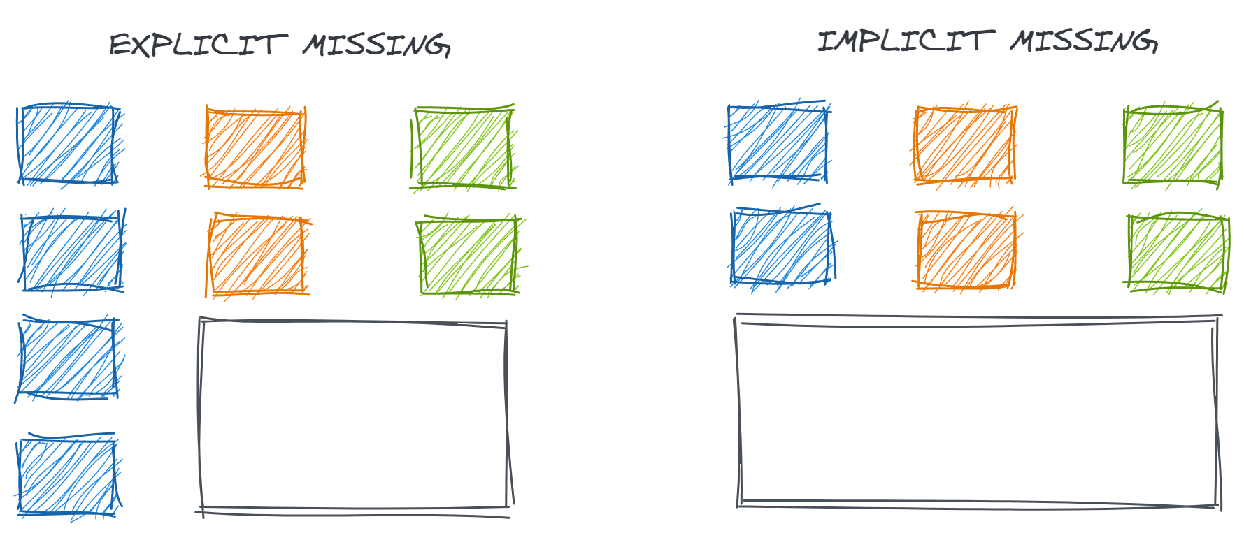
Another major encoding decision is how to handle null values. Previously, in the discussion of Data Collection, we considered the presence and absence of full records. However, when preparing data for analysis, both data produces and consumers need to decide how to cope with the presence or absence of individual fields.
If records contain some but not all relevant information, they may be published with explicitly missing fields or the full record may not be published at all. The difference between implicit and explicit missingness on the resulting data is illustrated in Figure 2.7.
Understanding what the system implies by each explicitly missing data field is also critical for validation and analysis. Checks for data completeness usually include counting null values, but null data isn’t always incorrect. In fact, null data can be highly informative if we know what it means. Some meanings of null data might include:
-
Field is not relevant: Perhaps our
loginstable reports the mobile phone operating system (iOS or Android) that was used to access the login page to track platform-specific issues. However, there is no valid value for this -
Relevant value is not known: Our
loginstable might also have anaccount_idfield which attempts to match login attempts to known accounts/customers using different metadata like cookies or IP addresses. In theory, almost everyone trying to log in should have an account identifier, but our methods may not be good enough to identify them in all cases -
Relevant value is null: Of course, sometimes someone without an account at all might try to log in for some reason. In this case, the correct value for an
account_idfield truly is null - Relevant value was recorded incorrectly: Sometimes systems have glitches. Without a doubt, every single login attempt should have a timestamp, but such a field could be null if this data was somehow lost or corrupted at the source
Similarly, different systems might or might not report out these nulls in different ways such as:
- True nulls: Literally the entry in the resulting dataset is null
-
Null-like non-nulls: Blank values like an empty string (
'') that contain a null amount of information but won’t be detected when counting null values -
Placeholder values: Meaningless values like an
account_idof00000000for all unidentified accounts which preserve data validity (the expected structure) but have no intrinsic meaning -
Sentinel/shadow values: Abnormal values which attempt to indicate the reasons for null-ness such as an
account_idof-1when no browser cookies were found or-2when cookies were found but did not help link to any specific customer record
Each of these encoding choices changes the definitions of appropriate completeness and validity for each field and, even more critically, impacts the expectations and assertions we should form for data accuracy. We can’t expect 100% completeness if nulls are a relevant value; we can’t check validity of ranges as easily if sentinel values are used with values that are outside the normal range (hopefully, or we have much bigger problems!) So, understanding how upstream systems should work is essential for assessing if they do work.
Similarly, understanding how our null data is collected has significant implications for how we subsequently process it. We will discuss this more in Chapter -Chapter 3 (Computational Quandaries).
2.4.2 Data Transformation
Finally, once the data is roughly where we want it, it likely undergoes many transformations to translate all of the system-generated fields we discussed in data collection into semantically-relevant dimensions for analytical consumers. Of course, the types of transformations that could be done are innumerable with far more variation than data loading. So, we’ll just look at a few examples of common failure patterns.
2.4.2.1 Pre-Aggregation
Data transformations may include aggregating data up to higher levels of granularity for easier analysis. For example, a transformation might add up item-level purchase data to make it easier for an analyst to look at spend per order of a specific user.
Data transformations not only transform our data, but they also transform how the dimensions of data quality manifest. If data with some of the completeness or uniqueness issues we discussed with data loading is pre-aggregated, these problems can turn into problems of accuracy. For example, the duplicate or partial data loads that we discussed when aggregated could suggest inaccurately high or low quantities respectively.
2.4.2.2 Field Encoding
When we assess data consistency across tables,
Categorical fields in a data set might be created in any number of ways including:
- Directly taken from the source
- Coded in a transformation script
- Transformed with logic in a shared user-defined function (UDFs) or macro
- Joined from a shared look-up table
Each approach has different implications on data consistency and usability.
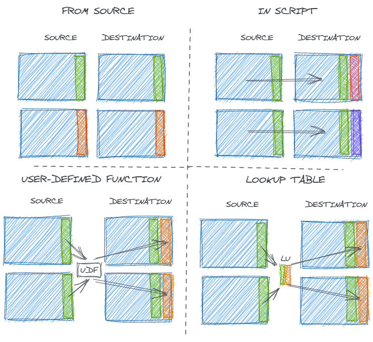
Using fields from the source simply is what it is – there’s no subjectivity or room for manual human error. If multiple tables come from the same source, it’s likely but not guaranteed that they will be encoded in the same way.
Coding transformations in the ELT process is easy for data producers. There’s no need to coordinate across multiple processes or use cases, and the transformation can be immediately modified when needed. However, that same lack of coordination can lead to different results for fields that should be the same.
Alternatively, macros, UDFs, and look-up tables provided centralized ways to map source data inputs to desired analytical data outputs in a systemic and consistent way. Of course, centralization has its own challenges. If something in the source data changes, the process of updating a centralized UDF or look-up table may be slowed down by the need to seek consensus and collaborate. So, data is more consistent but potentially less accurate.
Regardless, such engineered values require scrutiny – particularly if they are being used as a key to join multiple tables – and the distinct values in them should be carefully examined.
2.4.2.3 Updating Transformations
Of course, data consistency is not only a problem across different data sources but within one data source. Regardless of the method of field encoding used in the previous step, the intersection of data loading and data transformation strategies can introduce data consistency errors over time.
Often, for computation efficiency, analytical tables are loaded using an incremental loading strategy. This means that only new records (determined by time period, a set of unique keys, or other criteria) from the upstream source are loaded to the downstream table. This is in contrast to a full refresh where the entire downstream table is recreated on each update.
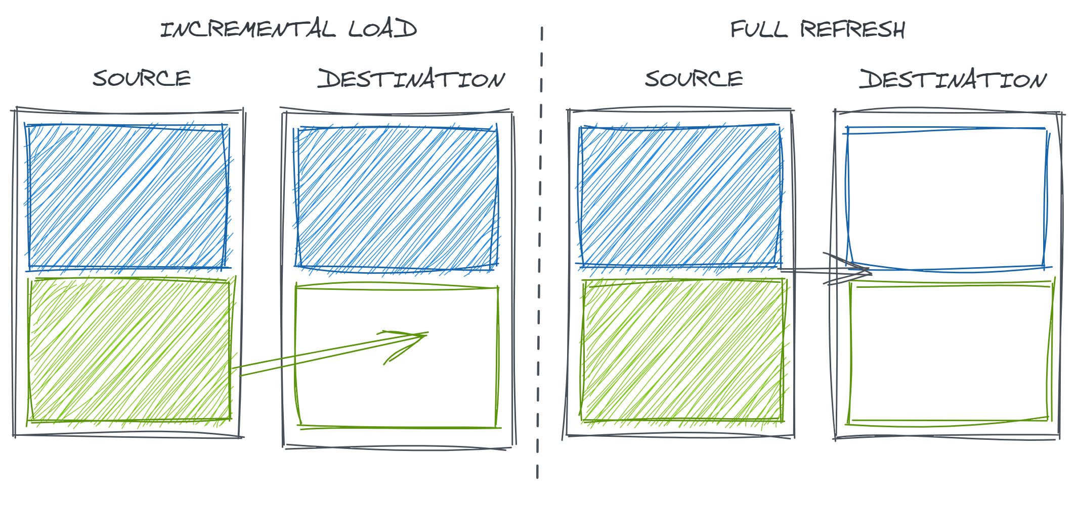
Incremental loads have many advantages. Rebuilding tables in entirety can be very time consuming and computationally expensive. In particular, in non-cloud data warehouses that are not able to scale computing power on demand, this sort of heavy duty processing job can noticeably drain resources from other queries that are trying to run in the database. Additionally, if the upstream staging data is ephemeral, fully rebuilding the table could mean failing to retain history.
However, in the case that our data transformations change, incremental loads may introduce inconsistency in our data over time as only new records are created and inserted with the new logic.
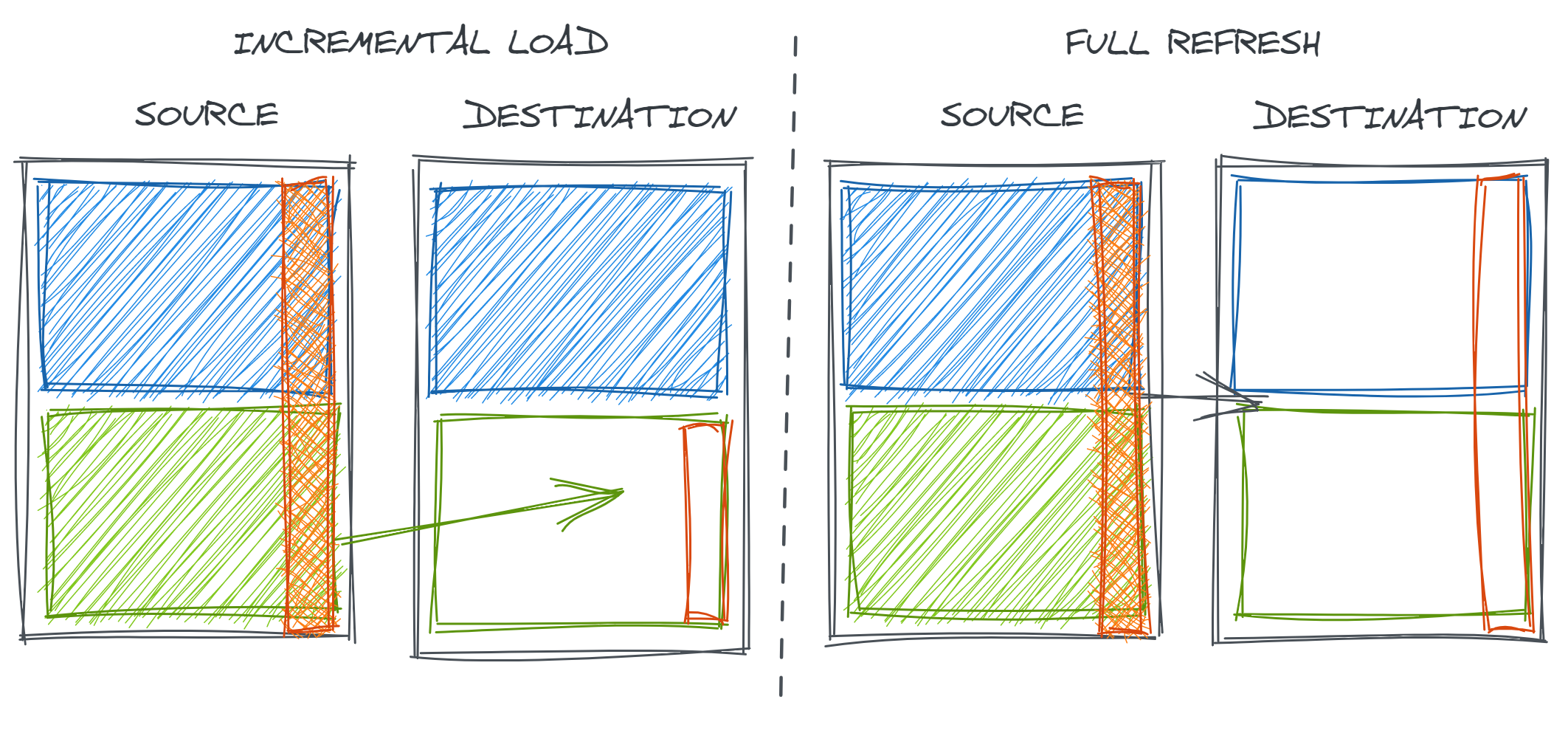
This is also a problem more broadly if some short-term error is discovered either with data loading or transformation in historical data. Incremental strategies may not always update to include the corrected version of the data.
Regardless, this underscores the need to validate entire datasets and to re-validate when repulling data.
2.5 More on Missing Data (TODO)
MCAR / MAR / MNAR
2.6 Other Types of Data (TODO)
2.6.1 Survey Data
2.6.2 Human-Generated
2.7 Strategies (TODO)
2.7.1 Understand the intent
- Why was data originally collected? By whom and for what purpose?
- Are there clear, unique definitions of key concepts (e.g. entites, measures)? What are they?
- Documentation (metadata, dictionaries)
2.7.2 Understand the execution
- learn about the real-world systems
- understand key steps in data production process
- documentation (lineage, provenance)
2.7.3 Seek expertise
- talking to experts (upstream and downstream)
2.7.4 Trust but verify
- always on data validation
- summaries
- context-informed assertions
- exploratory analysis
2.8 Real World Disasters
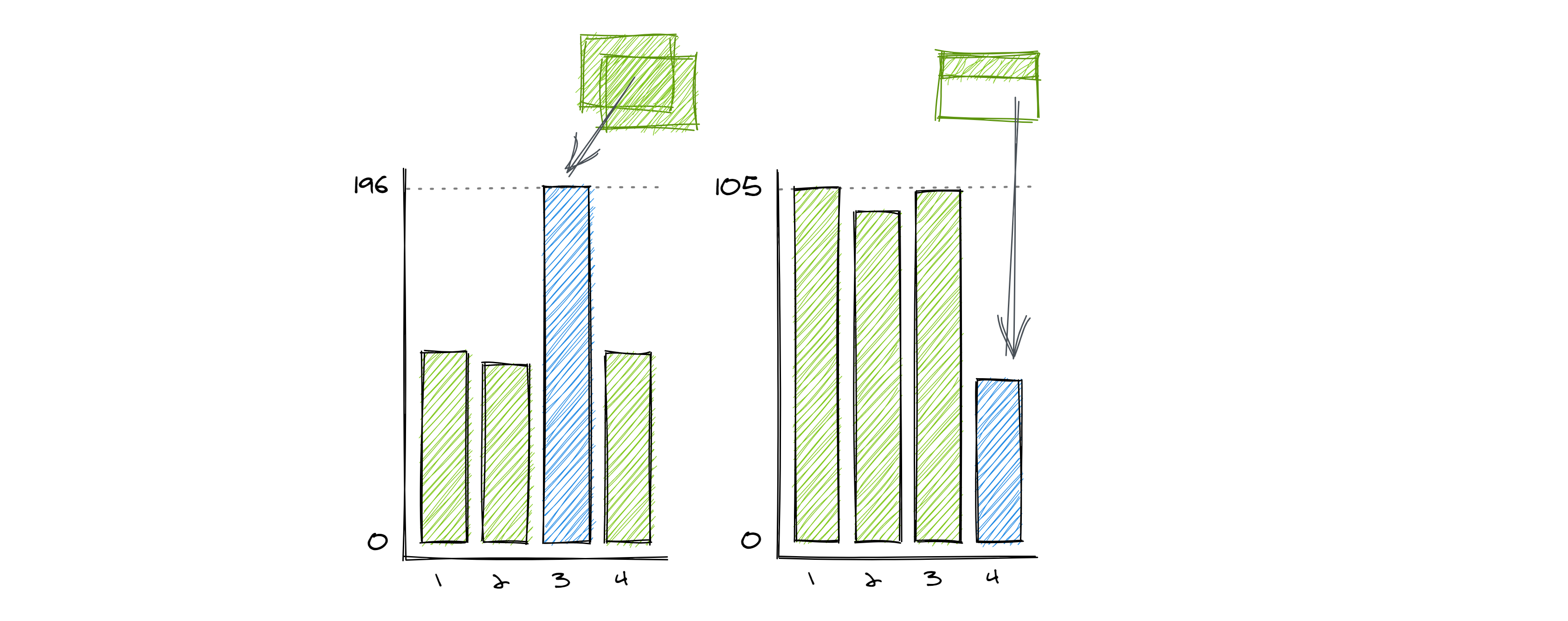
2.8.1 Data loading artificially spikes COVID cases
Data loading, particularly when a new process is introduced can go astray and lead to spurious results. The city of El Paso discovered this after reporting an exceedingly high number of daily COVID cases (Borunda 2020):
El Paso city and public health officials on Thursday admitted to a major blunder, saying that the more than 3,100 new cases reported a day earlier was incorrect.
The number was the result of a two-day upload of cases in one day after the public health department went from imputing data manually to an automatic data upload that was intended to increase efficiency, Public Health Director Angela Mora said at news conference.
This instance demonstrates not only how data goes wrong but also how easy it is to trust discrepancies and find explanations in real-world phenomena. The article goes on to suggest that the extremely high case numbers were not immediately caught given the overall “alarming” levels:
Mora said she accepted responsibility and that she should have taken a deeper look after noticing the abnormally high number of new cases.El Paso County is still seeing more than 1,000 new cases on a daily basis, officials said. The correct number of new cases Wednesday was 1,537.
“The numbers are still high and they are still alarming but they were not as high as we reported,†Mora said.
Similar data artifacts also arose from a variety of other factors besides system changes. For example, delays in 9-to-5 office paperwork (the real-world events triggering the creation of some key data elements) over the holidays led to more artificial trends in data reporting around the end-of-year holidays:
While 238 deaths is the most reported in Illinois since the start of the pandemic, the IDPH noted in its release that some data was, “delayed from the weekends, including this past holiday weekend.â€
- Illinois sees biggest spike in reported COVID-19 deaths to date after holidays delay some data, officials say, WGN9 (TODO CITATION)
2.8.2 Data encoding leads to incorrect BMI calculation
Data that is encoded inconsistently may be mishandled in automated decision processes. For example, data manually entered into electronic health records (EHR) by countless care provides might be compiled into a single source although the meanings could be inconsistent.
In the early days of the COVID19 vaccination push, some regions chose to prioritize their vaccine supply by certain individual characteristics including a high body mass index (BMI), which is a function of one’s weight relative to their height.
One 6ft 2in tall man’s data was misinterpreted to suggest that he was 6.2 centimeters tall; this caused his to get high priority for a vaccine.
As described in the BBC (“Covid: Man Offered Vaccine After Error Lists Him as 6.2cm Tall” 2021):
A man in his 30s with no underlying health conditions was offered a Covid vaccine after an NHS error mistakenly listed him as just 6.2cm in height. Liam Thorp was told he qualified for the jab because his measurements gave him a body mass index of 28,000.
TODO: Data Smells Code https://arxiv.org/pdf/2203.08007.pdf
TODO: Data missing from COVID research https://journals.plos.org/plosone/article?id=10.1371/journal.pone.0248793