3 Computational Quandaries (WIP)
After gaining confidence in one’s data (or, at least, making peace with it), the next step in a data analysis is often to start cleaning and exploring that data with summary statistics, plots, and models. Generally, this requires a computational tool like SQL, R, or python.
The process of computation itself can be fraught with challenges. Computational tools are extremely literal; they are excellent at doing precisely what they were told to do but not often what analysts might have meant or wished that they would do. Additionally, the moment an analyst begins to use a tool, the conversation is no longer between them and the data; suddenly, the mental model of how every single tool developer thought you might want to do analysis affects the tools’ behaviors and the analysts’ results.
In this chapter, we will explore common ways that tools may do something technically correct, reasonable, and as-intended but very much not what analysts may expect. Along the way, we will see how computational methods interact with the data encoding choices we discussed in Chapter 2 (Data Dalliances).
3.1 Preliminaries - Data Computation
Before we think about specific tools or failure modes, we can first consider the common types of operations that the analytical tools allow us to do with our data.
3.1.1 Single Table Operations
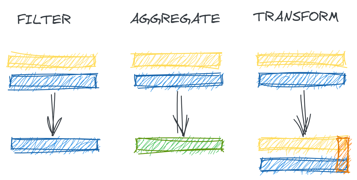
Given a single data table, we may wish to do operations (illustrated in Figure 3.1) such as:
- Filtering: Extracting a subset of a dataset for analysis based on certain inclusion criteria for each record
- Aggregation: Grouping our data table by one or more variables and condensing information across records with aggregate functions like counts, sums, and averages
- Transformation: Create new columns or modifying existing columns to represent more complex or domain-specific context
3.1.2 Multiple Table Operations
Often, we can get additional value in an analysis by combining multiple types of information from difference tables. When working with multiple tables, we may be interested in:
- Combining Row-wise: Taking multiple tables with the same schemas (column names and data types) and creating a single table which contains the union (all records), intersection (only matching), or difference (only in one) of the records in the two tables
- Combining Column-wise: Appending additional fields to existing records through joining (also known as merging) multiple tables
3.1.3 Mechanics
All of these operations rely on a few core computational tasks:
- Arithmetic: Basic addition, subtraction, multiplication, and division to aggregate and transform data
- Mapping: Similar to arithmetic, other one-to-one or many-to-one transformations of numerical or categorical data (such as binning into categories)
- Equality: Comparing whether or not two values are equal is critical for data filtering, column-wise combination, and certain types of data transformation
- Casting: Converting data types of different elements into a comparable format is necessary for row-wise combination and often a prerequisite to certain equality and arithmetic tasks
While these operations may seem simple, their behavior within certain tools and when employed for certain data types may sometimes lead to unintuitive or misleading results.
3.2 Null Values
In Chapter 2 (Data Dalliances), we discuss how null values may represent many different concepts and be encoded in multiple different ways. In addition to those semantic challenges, various representations of null values may cause different computational problems.1 In this section, we will explore these potential failure modes.
3.2.1 Types of Null Values
Not only can null values represent many different things (as explored in Chapter 2), they also may be represented in many different ways. Understanding how nulls are encoded in one’s dataset is a critical prerequisite to attempting any of the computations described in the subsequent sections.
3.2.1.1 Language representations
Different programming languages each offer their own versions of null values – and sometimes more than one. For example, the R language includes NA, typed NAs (e.g. NA_integer_, NA_character_), NaN, and NULL; meanwhile, core python has None and the numpy module provides a nan.
These different values carry different semantic and functional meanings. For example R’s NA generally means “the presence of an absence” whereas NULL is “the absence of a presence”. This is articulated more clearly if we examine the lengths of these objects and observe that NA has a length 1 whereas NULL has a length 0.
is.finite(NA)
is.infinite(NA)
[1] FALSE
[1] FALSEAs further proof that these are not interchangeable, we may use the helper functions is.na() and is.null(). It’s false that NA is NULL and essentially unable to be evaluated if NULL is NA because NULLs are truly nothing.2
To further complicate matters, we have NaN (“not a number”), along with -Inf and Inf, which generally arise when we attempt to abuse R’s calculator. Somewhat charmingly, Inf and -Inf may be used in some rudimentary calculations where the limit is returned.3
1/0
0/0
1/Inf[1] Inf
[1] NaN
[1] 03.2.1.2 Sentinel value encoding
Beyond these null types offered natively by different programming languages, there are also many different data management conventions for null values. Because null values can have many meanings, sometimes missing fields are encoded with “out of range” values which intend to suggest a type of missingness.
For example, the US Census Bureau’s Medical Expenditure Panel Survey uses the following reserved codes to denote different types of missingness: (TODO: cite p10 https://www.meps.ahrq.gov/data_stats/download_data/pufs/h206a/h206adoc.pdf)
- -1 INAPPLICABLE Question was not asked due to skip pattern
- -7 REFUSED Question was asked and respondent refused to answer question
- -8 DK Question was asked and respondent did not know answer
- -14 NOT YET TAKEN/USED Respondent answered that the medicine has not yet been used
- -15 CANNOT BE COMPUTED Value cannot be derived from dataThis approach preserves a lot of relevant information while, at the same time, being readily apparent that these values are not valid when the data is manually inspect. Unfortunately, manually inspecting every data field is rarely possible, and such sentinel values may go undetected when looking at higher-level summaries.
Consider a survey of a population of retired adults where age is coded as 999 if not provided. Below, we simulate 100,000 such observations that are uniformly distributed between the age of 65 and 95 (hence, have an expected value of 80). Next, we replace merely half of a percent with our “null” values of 999. Taking the mean with these false values results in a mean of about 85. This number alone might not raise the alarm; after all, we know the dataset’s population is older adults. However, accidentally treating these as valid values biases our results by a somewhat remarkable five years.
set.seed(123)
n <- 100000
p <- 0.01 / 2
ages <- runif(n, 65, 95)
ages_nulls <- ages
ages_nulls[1:(n*p)] <- 999
mean(ages)
mean(ages_nulls)[1] 79.97897
[1] 84.57468So, the first order of business with null values is understanding how they are encoded and translating them to the most computationally appropriate form. However, that is only the beginning of the story.
3.2.1.3 Other types of nulls (TODO)
might be blank string which won’t get detected in standard null checks
x <- ""
is.na(x)[1] FALSEsame thing is true in dataframes
library(dplyr)
df <- data.frame(x = c("a", "b", "", "d"))
summarize_all(df, ~sum(is.na(.))) x
1 0in such cases, need to explicitly check for such alternative encodings like blank strings
x <- ""
is.na(x) | x == ""[1] TRUEof course, a blank string isn’t the only choice
could also have an empty string of any length
[1] FALSE
[1] TRUE
[1] TRUEwe’ll see more about how fluid strings can be in the string section below
3.2.2 Aggregation
Once null values are coded as “true” nulls, how these nulls are handled in the simple aggregation of data varies both across different languages and across different functions within a language. To better understand the problems this might cause, we will look at examples in R and SQL.
To explore aggregation, let’s build a simple dataset. We will suppose that we are working with a subscription-based e-commerce service and that we are looking at a spend dataset with one record per customer and information about the amount they spent and returned in a given month:
spend <-
data.frame(
AMT_SPEND = c(10, 20, NA),
AMT_RETURN = as.numeric(rep(NA, 3))
)
head(spend) AMT_SPEND AMT_RETURN
1 10 NA
2 20 NA
3 NA NATo compute the average amount spent (AMT_SPEND) with the dplyr package, an analyst might first reasonably write the following summarize() statement. However, as we can see, due to the presence of null values within the AMT_SPEND column, the result of this aggregation is for the whole quantity of AVG_SPEND to be set to the value NA.
A glance at the documentation for the mean() function4 reveals that the function has a parameter called na.rm. This parameter’s default value is FALSE, but, when it is set to TRUE, it removes null values from our dataset. Adding this argument to the previous statement allows us to reach a numerical answer.
AVG_SPEND AVG_SPEND_NARM
1 NA 15However, is this the right numerical answer? Recall that what na.rm = TRUE does is drop the null values from the set of numbers being averaged. However, suppose the null values represent that no purchases were made for a given customer in a given month. That is, zero dollars were spent. In effect, we have removed all non-purchasers from the data being averaged.
More precisely, we have switched from taking the average
\[ \frac{ \sum_{1}^{n} Spend }{\sum_{1}^{n} 1} \] over all \(n\) customers
to taking the average
\[ \frac{ \sum_{Spend > 0} Spend }{\sum_{Spend > 0} 1} \] over only those customers with spend.
At face value, we could say that the code above is giving the incorrect answer; by dropping some low (zero) purchase amounts, the average amount spend per customer is inflated. A second perspective, which is someone more philosophically troubling, is that this tiny change to the code which fixed the obvious problem (returning a null value) has introduced a non-obvious problem by fundamentally changing the question that we are asking. By dropping all accounts from our table who made no purchases, we are no longer answering “What is the average amount spent by all of our customer?” but rather “What is the average amount spent by an actively engaged customer?” In the language of probability theory, we might say that we have then changed our estimand from the expected value of spend to expected value of spend conditional on spend being positive. This technical quirk has significant analytical impact.
To answer the real question at hand, we have a couple of options. We could manually sum() the amount spent with the option to drop nulls but then divide by the correct denominator (all observations – not just those with spend) or we could explicitly recode null values in AMT_SPEND to zero before taking the average.5 Either of these options lead to the correct conclusion of a lower average spend amount.
summarize(
spend,
AVG_SPEND_MANUAL = sum(AMT_SPEND, na.rm = TRUE) / n(),
AVG_SPEND_RECODE = mean(coalesce(AMT_SPEND, 0))
) AVG_SPEND_MANUAL AVG_SPEND_RECODE
1 10 10This is all well and good if we could just accept that the behaviors above are simply how nulls work, but further complexity comes as we see that there is no industry standard across tools. For example, as the SQL code below shows, SQL’s avg() function behaves more like R’s mean() with the na.rm = TRUE option set (whereas, you may recall that R’s mean() behaves with na.rm = FALSE by default). That is, the default behavior of SQL is to only operate on the valid and available values. The result of this default may mean that it is less obvious when our dataset has null values. SQL, unlike R, does not ask for “permission” to drop out nulls; instead, it unilaterally makes a decision how to handle these variables.
SELECT
avg(amt_spend) as AVG_SPEND
FROM spend AVG_SPEND
1 15However, this is not to suggest that null values cannot also be “destructive” in SQL (that is, returning null). While aggregation functions (which compute over the rows/records) like sum() and avg() drop nulls, operators like + and - (which compute across columns/variables in the same row/record) do not exhibit the same behavior. Consider, for example, if we wish to calculate the average net purchase amount (purchases minus returns) instead of the gross (total) purchase amount.
SELECT
avg(amt_spend - amt_return) as AVG_SPEND_NET
FROM spend AVG_SPEND_NET
1 NADespite what we learned above about SQL’s avg() function, the query above returns only a null value. What has happened? In our spend dataset, the amt_return column is completely null (representing no return purchases). Because the subtraction occurs before the average is taken, subtracting null values in the amt_return variable from valid numbers in amt_spend variable creates a new variable of all null values. This new variable, which is already all null, is passed to the avg() function. This process is shown step-by-step below.
SELECT
amt_spend,
amt_return,
amt_spend-amt_return
FROM spend AMT_SPEND AMT_RETURN amt_spend-amt_return
1 10 NA NA
2 20 NA NA
3 NA NA NA3.2.3 Comparison
Null values don’t just introduce complexity when doing arithmetic. Difficulties also arise any time multiple variables are assessed for equality or inequality. Since a null value is unknown, most programming languages generally will not consider nulls to be comparable with other nulls.
We can observe simple examples of this in both R and SQL. In neither language can a null value be assessed for equality or inequality versus either another number or another null.
NA == 3
NA > 10
NA == NA[1] NA
[1] NA
[1] NASELECT
(NULL = 3) as NULL_EQ_NUM,
(NULL > 10) as NULL_GT_NUM,
(NULL = NULL) as NULL_EQ_NULL NULL_EQ_NUM NULL_GT_NUM NULL_EQ_NULL
1 NA NA NAIn these toy examples, such outcomes may seem perfectly logical. However, this same reasoning can arise in sneakier ways and lead to uninteded results when equality evaluations are implicit in the task at hand instead of the singular focus. We’ll now see examples from data filtering, joining, and transformation.
If you’re familiar with SQL, you may have been surprised to notice that there is no FROM clause in the query above. In fact, SQL queries can treat values just like variables containing only a single record.
We will use this trick throughout the chapter for exploring how SQL works when we don’t have an ideal sample dataset to test certain scenarios. Beyond exposition in this book, this trick is also useful in practice.
3.2.3.1 Filtering
Suppose we want to split our dataset into two datasets based on high or low values of spend. We might assume the following two lines of code will create a clear partition (implying that each record would fall into exactly one group.)
However, if we examine the resulting datasets, we see that neither contains the third record which had a null value for the AMT_SPEND variable.
spend_lt20 AMT_SPEND AMT_RETURN
1 10 NAspend_gte20 AMT_SPEND AMT_RETURN
1 20 NAThe same situation results in SQL.
SELECT *
FROM spend
WHERE AMT_SPEND < 20 AMT_SPEND AMT_RETURN
1 10 NASELECT *
FROM spend
WHERE AMT_SPEND >= 20 AMT_SPEND AMT_RETURN
1 20 NAThis is a direct result of the fact that nulls cannot be compared for equality any inequality. We can think of data filtering as a two-step process: first evaluate whether the condition is TRUE or FALSE, then return only the records for which the condition holds true. When we conduct the more manual process of filtering step-by-step, we see that the null value of AMT_SPEND does not get a “truth value” when compared with a number. Thus, it is not contained in either “truth value” subset.
mutate(spend, is_lt20 = (AMT_SPEND < 20)) AMT_SPEND AMT_RETURN is_lt20
1 10 NA TRUE
2 20 NA FALSE
3 NA NA NAThus, whenever our data has null values, the very common act of data filtering risks excluding important information.
3.2.3.2 Joining
The same phenomenon as described above also happens when joining multiple datasets.
Suppose we have multiple datasets we wish to merge based on columns denoting a record’s name and date of birthday. For ease of exploration, we will make the simplest possible such dataset and simply try to merge it to itself. (This may seem silly, but often when trying to understand computationally complex things, it is a good idea to make the scenario as simple as possible. In fact, this idea is core to the concept of computational unit tests which we will discuss at the end of this chapter.)
bday <- data.frame(NAME = c('Anne', 'Bob'), BIRTHDAY = c('2000-01-01', NA))
bday NAME BIRTHDAY
1 Anne 2000-01-01
2 Bob <NA>In SQL, if we try to join this table, the records in row 1 will match because 'Anne' == 'Anne' and '2000-01-01' == '2000-01-01'. However, poor Bob’s record is eliminated because his birth date is logged as null, and NA == NA is false.
SELECT a.*
FROM
bday as a
INNER JOIN
bday as b
ON
a.NAME = b.NAME and
a.BIRTHDAY = b.BIRTHDAY NAME BIRTHDAY
1 Anne 2000-01-01In contrast, R’s dplyr::inner_join() function will not do this by default. This function lets us specifically control how nulls are matches with the na_matches argument, with a default option to match on NA values. (You may read more about the argument by typing ?dplyr::inner_join in the R console to pull up the documentation.)
inner_join(bday, bday, by = c('NAME', 'BIRTHDAY')) NAME BIRTHDAY
1 Anne 2000-01-01
2 Bob <NA>This example then is not only a cautionary tale for how null values may unintentionally corrupt our data transformations but also how “brittle” our knowledge and intuition may be when moving between tools. Neither of these default behaviors is strictly better or worse, but they are definitely different and have real implications on our analysis.
3.2.3.3 Transformation
A common task in data analysis is to aggregate results by subgroup. For example, we might want to summarize how many customers (rows/records) spent more or less than $10. To discern this, we might create a categorical variable for high versus low purchase amounts, group by this variable and count.
The psuedocode would read something like this:
data %>%
mutate(HIGH_LOW = << transform AMT_SPEND >>) %>%
group_by(HIGH_LOW) %>%
count()To define the HIGH_LOW variable, we might use a function like ifelse(), dplyr::if_else(), or dplyr::case_when(). However, once again, we have the issue of how values are partitioned when nulls are included. If we recode any records with AMT_SPEND of less than or equal to 10 to “Low” and default the rest to “High”, we will accidentally count all null values in the “High” group.
spend %>%
mutate(HIGH_LOW = case_when(
AMT_SPEND <= 10 ~ "Low",
TRUE ~ "High")
) %>%
group_by(HIGH_LOW) %>%
count()# A tibble: 2 x 2
# Groups: HIGH_LOW [2]
HIGH_LOW n
<chr> <int>
1 High 2
2 Low 1Instead, it is more accurate and transparent (unless we know specifically what null values mean and what group they should be part of) to not let one of our “core” categories by the “default” case in our logic. We can explicitly encode any residual values as something like “OTHER” or “ERROR” to help us see that there is a problem requiring extra attention.
spend %>%
mutate(HIGH_LOW = case_when(
AMT_SPEND <= 10 ~ "Low",
AMT_SPEND > 10 ~ "High",
TRUE ~ "OTHER")
) %>%
group_by(HIGH_LOW) %>%
count()# A tibble: 3 x 2
# Groups: HIGH_LOW [3]
HIGH_LOW n
<chr> <int>
1 High 1
2 Low 1
3 OTHER 1While nulls contribute to this issue, it’s important to realize that nulls are not the only factor causing this error nor or they the solution. The more substantial issue is the careless use of defaults and implicit encoding versus explicit encoding. In the second form of the SQL query above, we are more specific about exactly what is allowed in each category which ensures any unexpected inputs will not be allowed to “sneak” into ordinary outputs.
3.3 Logicals (TODO)
Much like the different versions of nulls that we met in the last section, logical data types use reserved keywords to represent TRUE and FALSE. (The exact formats of logical reserved keywords vary by language. R and SQL use TRUE and FALSE and python uses TRUE and FALSE.) This means that these names function like a number or a letter which intrinsically hold one specific value and cannot take on a different value besides their own.
TRUE = 5Error in TRUE = 5: invalid (do_set) left-hand side to assignment2 = 5Error in 2 = 5: invalid (do_set) left-hand side to assignmentAcross languages, TRUE and FALSE are considered equivalent to the numeric representations of 1 and 0 respectively.
as.numeric(TRUE)
as.numeric(FALSE)[1] 1
[1] 0A consequence of this numerical equivalency is that TRUE and FALSE may be compared to each other or other numbers and be included in mathematical expressions.
TRUE > FALSE
TRUE < 5
FALSE > -1
TRUE + 1
TRUE * 5[1] TRUE
[1] TRUE
[1] TRUE
[1] 2
[1] 5similar in SQL
select
TRUE > FALSE as a,
TRUE < 5 as b,
FALSE > -1 as c,
TRUE + 1 as d,
TRUE * 5 as e| a | b | c | d | e |
|---|---|---|---|---|
| 1 | 1 | 1 | 2 | 5 |
3.3.1 Language-specific nuances (CUT?)
3.3.1.1 Keyword abbrevations
R also recognizes the abbreviations of T and F as TRUE and FALSE respectively; however this is not recommended. T and F are not reserved keywords, so they can be overwritten with a different value. This makes code using such abbreviations “brittle” and less reliable.
if (T) {"Hello"} else {"Goodbye"}
if (F) {"Hello"} else {"Goodbye"}
T = 0
if (T) {"Hello"} else {"Goodbye"}[1] "Hello"
[1] "Goodbye"
[1] "Goodbye"3.3.1.2 Alternative representations
We’ve previously seen that logicals have associated numerical values. Different languages may also treat their string representations differently.
For example, R believes that the string "TRUE" is equal to the logical value TRUE when directly compared. However, this relationships breaks the transitive property of mathematics6 because TRUE equals both 1 and "TRUE", yet "TRUE" does not equal 1 so the mathematical operations that can be done with logical TRUE cannot be done with string "TRUE".
TRUE == 1
TRUE == "TRUE"
TRUE == "True"
TRUE * 5
"TRUE" * 5Error in "TRUE" * 5: non-numeric argument to binary operator[1] TRUE
[1] TRUE
[1] FALSE
[1] 5In contrast neither SQL not python honor the string forms of their respective logical reserved keywords at all.
select
(TRUE == 1) as is_int_true,
(TRUE == 'TRUE') as is_char_true,
TRUE*5 as true_times_five,
'TRUE'*5 as true_str_time_five is_int_true is_char_true true_times_five true_str_time_five
1 1 0 5 0True == 1
True == "True"
True == "TRUE"
True * 5
"True" * 5True
False
False
5
'TrueTrueTrueTrueTrue'3.3.2 Comparison (TODO)
The nuances of logical representation and handling seem straightforward in isolation. However, when encountered in real-world data problems, they are not isolated and are unlikely to be our main focus.
Imagine two datasets which all encode the same information but use boolean, string, and integer representations of a logical respectively.
df1 <- data.frame(ID = 1:3, IND = rep(TRUE, 3), X = 1:3)
df2 <- data.frame(ID = 1:5, IND = rep('TRUE', 5), Y = 11:15)
df3 <- data.frame(ID = 1:5, IND = rep(1, 5), Z = 21:25)By simple inspection, the logical and string representations in particular look superficially similar and yet they will behave differently.
head(df1) ID IND X
1 1 TRUE 1
2 2 TRUE 2
3 3 TRUE 3head(df2) ID IND Y
1 1 TRUE 11
2 2 TRUE 12
3 3 TRUE 13
4 4 TRUE 14
5 5 TRUE 15If we use R’s dplyr::filter() or base::subset() function to subset the data, the value of df1 will correctly subset based on the boolean values of IND. However, R will not know how to interpret the string version in df2.
Error in `filter()`:
! Problem while computing `..1 = IND`.
x Input `..1` must be a logical vector, not a character.subset(df2, df2$IND)Error in subset.data.frame(df2, df2$IND): 'subset' must be logical ID IND X
1 1 TRUE 1
2 2 TRUE 2
3 3 TRUE 3[1] ID IND X
<0 rows> (or 0-length row.names)
[1] ID IND Y
<0 rows> (or 0-length row.names)[1] ID IND Y
<0 rows> (or 0-length row.names)Error in `left_join()`:
! Can't join on `x$IND` x `y$IND` because of incompatible types.
i `x$IND` is of type <logical>>.
i `y$IND` is of type <character>>. ID IND X Y
1 1 TRUE 1 11
2 2 TRUE 2 12
3 3 TRUE 3 13select df1.*, df2.*
from
df1
left join
df2
on
df1.id = df2.id and
df1.ind = df2.ind| ID | IND | X | ID | IND | Y |
|---|---|---|---|---|---|
| 1 | 1 | 1 | NA | NA | NA |
| 2 | 1 | 2 | NA | NA | NA |
| 3 | 1 | 3 | NA | NA | NA |
import pandas as pd
data1 = {'ID': list(range(1, 4)),
'IND': [True] * 3,
'X': list(range(1,4))
}
data2 = {'ID': list(range(1, 6)),
'IND': ['True'] * 5,
'Y': list(range(11, 16))}
df1 = pd.DataFrame(data1)
df2 = pd.DataFrame(data2)
df1
df2 ID IND X
0 1 True 1
1 2 True 2
2 3 True 3
ID IND Y
0 1 True 11
1 2 True 12
2 3 True 13
3 4 True 14
4 5 True 15pd.merge(left = df1, right = df2, how = "left", on = ['ID', 'IND']) ID IND X Y
0 1 True 1 NaN
1 2 True 2 NaN
2 3 True 3 NaN
3.3.3 Logical Encoding (pandas case study)
https://twitter.com/pandas_dev/status/1579886907286491137?s=20&t=GXV9OMXUcJiPWyES6CUKoA
3.4 Numbers (TODO)
3.4.1 Integer division
In R (mostly what we’d expect)
1/2[1] 0.5ifelse(3/4 > 0.5, 'High', 'Low')[1] "High"In some SQL dialect SQL (SQLite shown. “Modern” interfaces like Snowflake and BigQuery don’t do this)
SELECT (1/2) as one_div_two one_div_two
1 0This rounding can get masked when we are recoding or doing subsequent calculations
SELECT
case
when 3/4 > 0.5 then 'High'
else 'Low'
end as high_low_int,
case
when 3.0 / 4 > 0.5 then 'High'
else 'Low'
end as high_low_float high_low_int high_low_float
1 Low HighThe above works because of implicit casting. We can also do explicit casting, but where we do this matters
SELECT
case
when cast(3 as float) / 4 > 0.5 then 'High'
else 'Low'
end as cast_first,
case
when cast(3/4 as float) > 0.5 then 'High'
else 'Low'
end as cast_last cast_first cast_last
1 High Low3.4.2 Inexact storage and comparison
In R
(3 - 2.9) <= 0.1
(2 - 1.9) <= 0.1
(1 - 0.9) <= 0.1[1] FALSE
[1] FALSE
[1] TRUE(3 - 2.9) == 0.1
(2 - 1.9) == 0.1
(1 - 0.9) == 0.1[1] FALSE
[1] FALSE
[1] FALSEdespite the fact that we see no difference
3 - 2.9
2 - 1.9
1 - 0.9[1] 0.1
[1] 0.1
[1] 0.1In python - same problem but in slightly different cases
(3 - 2.9) <= 0.1
(2 - 1.9) <= 0.1
(1 - 0.9) <= 0.1False
False
Truehere we can see the differences
3 - 2.9
2 - 1.9
1 - 0.90.10000000000000009
0.10000000000000009
0.09999999999999998Same thing with SQL where differences are masked
select
  3 - 2.9 as sub_three,
  2 - 1.9 as sub_two,
  1 - 0.9 as sub_one,
  (3 - 2.9) <= 0.1 as sub_compare_three,
  (2 - 1.9) <= 0.1 as sub_compare_two,
  (1 - 0.9) <= 0.1 as sub_compare_one
sub_three sub_two sub_one sub_compare_three sub_compare_two sub_compare_one
1 0.1 0.1 0.1 0 0 1Instead, can use either built-in equality checker (python equivalent is math.isclose) or check that difference between two numbers is in very small window
Another example
3.4.3 Division by zero
more of a design issue about the right way to handle
we’ve seen before how we have to understand other peoples use of null values
this is a case where we he to decide what makes most sense
3.5 Strings (WIP)
String data can be inherently appealing. At their best, strings are used to bring more readable and human interpretable values into a dataset. However, string data and the processing thereof comes with its own challenges.
First, unlike numbers, human language strings can be ambiguously defined. 2 is the only number to represent the value of two. However, the incorporation of human language means that many different words, phrases, and formatting choices can represent the same concept. This is confounded by instances where string data was manually entered, as is the case with user-input data.7
Secondly, string data is one of the most flexible datatypes and can contain any other types of information – from should-be-logical values ("yes"/"no", "true"/"false"), should-be-numeric values ("27"), should-be-date values ("2020-01-01"), and even complex data encodings like JSON blobs ("{"name":{"first":"emily","last":"riederer"},"social":{"twitter":"emilyriederer","github":"emilyriederer","linkedin":"emilyriederer"}}" with hideous formatting for emphasis.) For a data publisher, this may be a convenience, but as we will see it can turn into a frustration or a liability when functions and comparison operations are attempted with strings that semantically represent a different type of value.
3.5.1 Dirty Strings (TODO)
whitespace
"a" == "a"
"a b" == "a b"
"a b" == "a  b"
"a b" == "a b "
[1] TRUE
[1] TRUE
[1] FALSE
[1] FALSE“fancy” characters (alternate encodings like ms word)
' " ' == ' " '
' “ 'Å=='' " ' " '
[1] TRUE
[1] FALSEspecial characters and display versus values
x <- "a\tb"
cat(x) # what you see...
x == "a    b" # ...is not what you get
a b[1] FALSE3.5.2 Regular Expressions (TODO)
we promised not to be solution oriented, but
not knowing regex is a disaster when trying to work with string data…
3.5.3 Comparison
TODO
3.5.3.1 String ordering
Strings are ranked based on alphabetical order just like a dictionary. Some properties of this ordering include that:
- numbers are smaller than letters (
1 < "a") - lower-case is smaller than upper case (
"a" < "A") - fewer characters are smaller than more characters (
"a" < "aa")
Such rules make perfect sense for true characters. However, when strings are used as a “catch all” to represent other structures, typical comparison operators can produce odd results. For example, it is generally uncontroverisal that ninety-one is less than one hundred twenty. However, the string "91" is greater than "120" because only the character "9" is compared to the character "1".8
91 < 120
"91" < "120"
[1] TRUE
[1] FALSEWhen strings are used to represent dates and times, comparison operators may or may not work depending on the precise formatting conversions. Below, we see that “YYYYQQ”-formats sort correctly because the information is hierarchically nested; millenia are compared before centuries, centuries before decades, decades before years, and years before quarters. However, many other string representations of dates, like “QQ-YYYY” will not order correctly. Related topics will be discussed in the “Dates and Times” section.
"20190Q4" < "2020Q3" # string (alphabetic) ordering same as semantic ordering
"Q4-2019" < "Q3-2020" # string and semantic orderings are different
[1] TRUE
[1] FALSEThese examples demonstrate that we shouldn’t rely on sorting schemes that follow different rules. Before doing comparisons on such types, its a safer bet to cast them to the format most truly representative of their types. If, for some reason, you do wish to keep them as strings, the second example shows that its is wise to format them in the most conducive format possible so things just work.
3.5.3.2 Type coercion
We discussed string comparison before when looking at “dirty” strings. More unexpected behavior arises when strings are compared across different data types. Many computing programs will attempt to coerce the objects to a similar and comparable type. Sometimes, this can be convenient as operations “just work”, but as always there is a cost for convenience. As we’ll see, delegating important decisions to our computing engine may not always capture the semantic relationships that we are most interested in.
For example, consider compare a string and a number. To make them more comparable, R will convert them both to strings before checking for equality. Thus, the number 2020 is equivalent to the string "2020" but not the string "02020".
"2020" == 2020
"02020" == 2020
[1] TRUE
[1] FALSEIn contrast, SQLite9 thinks that the string '2020' is greater than the number 2020 and that these two quantities are not equal.
SELECT
  case when     '2020' =  2020 then 1 else 0 end as is_eq,
  case when not '2020' == 2020 then 1 else 0 end as not_eq,
  case when     '2020' <  2020 then 1 else 0 end as is_lt,
  case when     '2020' >  2020 then 1 else 0 end as is_gt
is_eq not_eq is_lt is_gt
1 0 1 0 1^TODO: where this could cause problems (FIPS example?)
3.5.4 Transformation (TODO)
basic things like addition differ by language
in R, returns error:
'a' + 'b'Error in "a" + "b": non-numeric argument to binary operator'a' * 5Error in "a" * 5: non-numeric argument to binary operatorin SQLite, goes to zero:
SELECT
  'a' + 'b' as string_add,
  'a'*5 as string_mult
string_add string_mult
1 0 0in python, does concatenation for + and analogous (concatenation of repeat) for *:
'a' + 'b''ab''a' * 5'aaaaa'3.6 Dates and Times (WIP)
Unlike character strings, dates and times seem like they should be well defined with distinct, quantifiable components like years, months, and days. However, many different conventions for date formatting and underlying storage formats exist. This leads to similar challenges with dates and times as we saw with strings before.
Some common formats in the wild are:
- YYYYMMDD
- YYYYMM
- MMDDYYYY
- DDMMYYYY
- MM/DD/YYYY
- MM/DD/YY
- DD/MM/YYYY
- YYYY-MM-DD (ISO8601)
In addition to how dates are formatted, they may be stored in a variety of different ways “under the hood” such as Unix time (seconds since 1970-01-01 00:00:00 UTC) and Julian time (days since noon in Greenwich on November 24, 4714 B.C) (TODO).
To complicate matters further, many of these formats may be represented either by native date types in various programs or by more basic data types (such as integers for the first four and strings for the last four). In addition, analogous formats exist for timestamps which encode both calendar date and time of day (hour, minute, and second information).
TODO: why ISO8601?
3.6.1 Comparison
Automatic conversion of data types Dates versus timestamps
df_dt <-
data.frame(
  DT_ENROLL = as.Date("2020-01-01"),
  DT_PURCH  = 20200101,
  DT_LOGIN  = as.POSIXlt("2020-01-01T12:00:00")
  )
none of these are equal so nothing returns on filtering
[1] 0Warning in mask$eval_all_filter(dots, env_filter): Incompatible methods
("Ops.Date", "Ops.POSIXt") for "=="[1] 0the same thing happens in sql
select * from df_dt where DT_ENROLL = DT_PURCH[1] DT_ENROLL DT_PURCH DT_LOGIN
<0 rows> (or 0-length row.names)select * from df_dt where DT_ENROLL = DT_LOGIN[1] DT_ENROLL DT_PURCH DT_LOGIN
<0 rows> (or 0-length row.names)in what way aren’t they equal? to understand this its helpful to know how the computer encodes these dates
with as.numeric() in R we can see the numeric representation of the date
as.numeric(df_dt$DT_ENROLL)[1] 18262this works the same way in SQL
select cast(DT_ENROLL as integer), cast(DT_PURCH as integer) from df_dt cast(DT_ENROLL as integer) cast(DT_PURCH as integer)
1 18262 20200101this has the implication that things that are on the same date have an inequality relationship in both languages
select
  cast(DT_ENROLL as integer),
  case when DT_ENROLL < 18000 then 1 else 0 end as lt_18000,
  case when DT_ENROLL < 19000 then 1 else 0 end as lt_19000,
  case when DT_ENROLL < DT_PURCH then 1 else 0 end as lt_purch
from df_dt
cast(DT_ENROLL as integer) lt_18000 lt_19000 lt_purch
1 18262 0 1 1Note this this can affect both filters and joins
and this similarly causes a more general problem when comparing a date to a date-as-an-integer
as.Date("2020-01-01") > 20160501[1] FALSEselect cast('2020-01-01' as date) > 20160501 cast('2020-01-01' as date) > 20160501
1 03.7 Changing Data Types (TODO)
data types can incidentally change between programs
df <- data.frame(DT = as.Date("2020-10-01"))
print("-- At creation --")
sprintf("Class of DT variable: %s", class(df$DT))
tmp <- tempfile()
write.csv(df, file = tmp, row.names = FALSE)
df <- read.csv(file = tmp)
print("-- After saving and reloading with read.csv --")
sprintf("Class of DT variable: %s", class(df$DT))
[1] "-- At creation --"
[1] "Class of DT variable: Date"
[1] "-- After saving and reloading with read.csv --"
[1] "Class of DT variable: character"some tools try to make “smart” guesses based on format
library(readr)

df <- readr::read_csv(file = tmp)
print("-- After saving and reloading with readr --")
sprintf("Class of DT variable: %s", class(df$DT))
[1] "-- After saving and reloading with readr --"
[1] "Class of DT variable: Date"however, this can make things slower or unideal (one example: https://github.com/tidyverse/readr/issues/1094#issuecomment-628612430). you can also specify your own types manually
3.8 Factors in R (TODO)
factor(c(0,1,0,1)) == 1
as.integer(factor(c(0,1,0,1))) == 1
as.integer(factor(c(0,1,0,1)))
[1] FALSE TRUE FALSE TRUE
[1] TRUE FALSE TRUE FALSE
[1] 1 2 1 23.9 Programming Errors (TODO)
3.9.1 Default Cases (WIP)
see case-when example in nulls section
3.9.2 Order of Operations (WIP)
PEMDAS but sometimes still ambiguous
1 + 1  * 2 / 3 - 1
(1 + 1) * 2 / 3 - 1
1 + 1 * 2 / (3 - 1)
[1] 0.6666667
[1] 0.3333333
[1] 2SQL clause order of evaluations
3.9.3 Object References (WIP)
Copying and modifying object overview
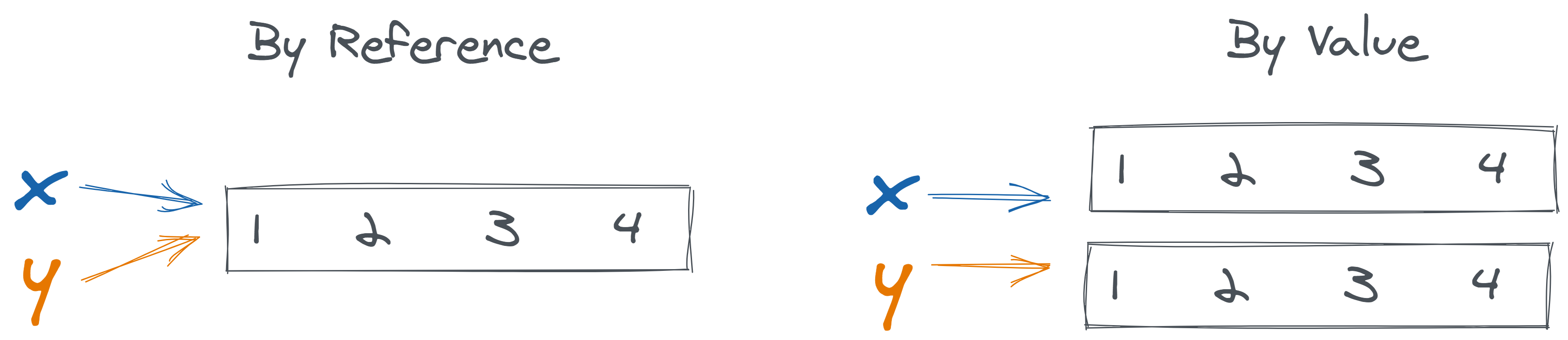
When might each be preferred?
What risks are there if we don’t understand which we are doing?
In Python
x = [1,2,3]
y = x
y.append(4)
print(y)
print(x)
[1, 2, 3, 4]
[1, 2, 3, 4]z = x.copy()
z.append(5)
print(z)
print(x)[1, 2, 3, 4, 5]
[1, 2, 3, 4]pandas DataFrame methods with inplace arg (False is default)
In R
library(data.table)

DT <- data.table(a=c(1,2), b=c(11,12))
print(DT)

newDT <- DT        # reference, not copy
newDT[1, a := 100] # modify new DT

print(DT)          # DT is modified too.

DT = data.table(a=c(1,2), b=c(11,12))
newDT <- DT
newDT$b[2] <- 200  # new operation
newDT[1, a := 100]

print(DT)
a b
1: 1 11
2: 2 12
a b
1: 100 11
2: 2 12
a b
1: 1 11
2: 2 12From https://stackoverflow.com/questions/10225098/understanding-exactly-when-a-data-table-is-a-reference-to-vs-a-copy-of-another
import pandas as pd

# set-up sample data ----
data = {'a': [1, 2],
        'b': [11, 12]}
df = pd.DataFrame(data = data)

# rename columns without replacing ----
df.rename(columns = {'a':'x'})
x b
0 1 11
1 2 12df
# rename columns with replacing ---- a b
0 1 11
1 2 12df.rename(columns = {'a':'x'}, inplace = True)
df x b
0 1 11
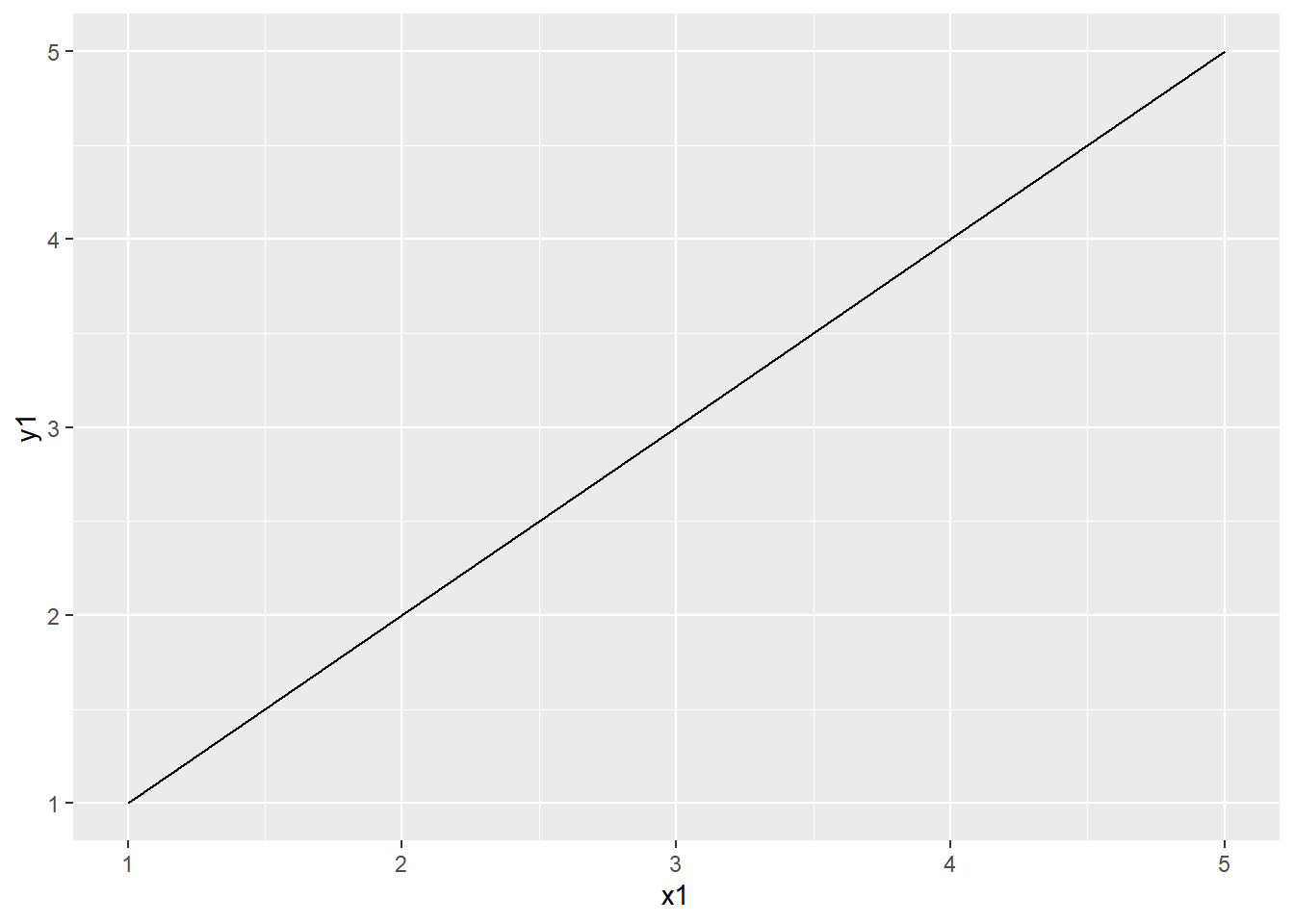
1 2 12add_ones <- function(data) {
data$x0 <- rep(0, nrow(data))
}
df <- data.frame(x1 = 1:5)
df x1
1 1
2 2
3 3
4 4
5 5add_ones(df)
df x1
1 1
2 2
3 3
4 4
5 5add_ones <- function(data) {
data$x0 <- rep(0, nrow(data))
return(data)
}
df <- data.frame(x1 = 1:5)
df x1
1 1
2 2
3 3
4 4
5 5add_ones(df) x1 x0
1 1 0
2 2 0
3 3 0
4 4 0
5 5 0df x1
1 1
2 2
3 3
4 4
5 5df2 <- add_ones(df)
df2 x1 x0
1 1 0
2 2 0
3 3 0
4 4 0
5 5 03.10 Trusting Tools
3.10.1 Delegating decisions
A theme throughout this book is the fundamentally social nature of data analysis. Data analysis is fraught without understanding the countless decisions made along the way by those who generated it (whose data is reflected), those who collected it, those who migrated it, and those who have posed questions of it. On one hand, this is a beautiful aspect of analysis; on the other hand, it means that analysts and their analyses are subject to all of the cognitive and social psychological biases of everyday humans.
One such bias is “social proof”: assuming that if a tool behaves a certain way, it must be because it is correct.
Assuming that our tools know best is admittedly an attractive proposition. It appeals to a desire to think that someone, somewhere is “in charge” and, perhaps more critically, helps us avoid a domino effect of distrust (If we don’t trust our tools how can we trust our results? And if we can’t trust our results, how can we trust anything at all?) Unfortunately, there are many reasons are tools might not know best. For example, the tool’s developer might have:
- Made a mistake
- Had a different analysis problem in mind with a different optimal approach
- Been optimizing for a different constraint (e.g. explainability vs. accuracy, speed vs. theoretical properties)
- Come from a community with different norms
- Been affording users the flexibility to do things many ways even if they don’t agree
- Built a certain feature for a different purpose than how you are using it
- Not thought about it at all
As a few concrete examples from popular open source tools. We’ll look briefly at the prominent python library scikitlearn for machine learning and Apache Spark, an engine for large-scale distributed data processing.
3.10.1.1 Defaults in scikitlearn
scikitlearn’s default behavior for logistic regression modeling10 automatically applies L2 regularization. You might or might not know what this means, and you might or might not want to apply it to your problem. That’s fine. The important thing is that it will change your estimates and predictions, and it is not a part of the classical definition of that algorithm (for modelers coming from a statistical background.)
Of course, there’s nothing inherently wrong about this choice; the library authors just had different goals than a typical statistical. scikitlearn developer Olivier Grisel explains on Twitter that this choice (and others in the library) is explained because “Scikit-learn was always designed to make it easy to get good predictive accuracy (eg as measured by CV) rather than as statistical inference library.” Additionally, this choice is documented in bold in the function documentation.
However, an analyst could easily miss this nuance if they do not read the documentation. Or, if they misinterpret this choice as social proof that regularization is always the right approach, they might not make the best choice for their own analysis.
3.10.1.2 Algorithms in Spark
As a second example, according to a 2015 Jira ticket, developers of Spark considered multiple methodologies they could use when adding the functionality to compute feature importance for a random forest. Ultimately, a core contributor advised against permutation importance due to its computational cost.
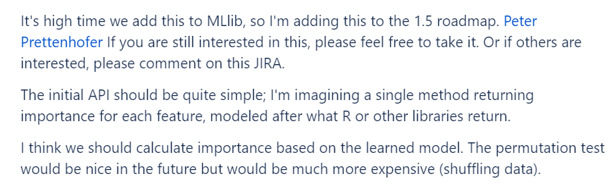
Clearly, no one wants a workflow that is too costly or timely to run. So, once again, there is no right or wrong. However, since every approach to feature importance has its own biases, pitfalls, and challenges in interpretation, it’s a mistake for an end-user to not carefully understand which algorithm is used and why.
3.10.1.3 Null handling in ggplot2 (TODO)
3.10.1.4 Boxplots in ggplot2 (TODO)
depending on how you change the scale it also changes the calculations
https://stackoverflow.com/questions/5677885/ignore-outliers-in-ggplot2-boxplot
3.10.2 “Off-Label” Use (TODO)
coined in https://www.rstudio.com/resources/rstudioglobal-2021/maintaining-the-house-the-tidyverse-built/
3.10.3 Security (TODO)
namespace squatting
executable code
3.11 Inefficient Processing (TODO)
3.12 Strategies (WIP)
Paragraph 1 TODO
Some computational quandaries are inherent to our tools themselves, but often they are a function both of the tools and the ways we chose to use them. More strategies related to writing robust and resilient code will be discussed in Chapter 11 (Complexify Code).
3.12.1 Understand the intent
- read the docs
- look at examples
- don’t carry default knowledge between languages
3.12.2 Understand the execution
- test out simple examples (like we’ve been doing)
- specificlly try out corner cases
3.12.3 Be explicit not implicit
- default arguments
- examples above with casting, coalescing
3.13 Real World Disasters (WIP)
https://www.theguardian.com/politics/2020/oct/05/how-excel-may-have-caused-loss-of-16000-covid-tests-in-england
The data error, which led to 15,841 positive tests being left off the official daily figures, means than 50,000 potentially infectious people may have been missed by contact tracers and not told to self-isolate.
https://journals.plos.org/ploscompbiol/article?id=10.1371/journal.pcbi.1008984
The Excel gene error has not been corrected